Sound Field Synthesis Toolbox for Python

Python implementation of the Sound Field Synthesis Toolbox.

Documentation:

http://sfs.rtfd.org/

Code:

http://github.com/sfstoolbox/sfs-python/

Python Package Index:

http://pypi.python.org/pypi/sfs/

Requirements

Obviously, you’ll need Python. We normally use Python 3.x, but it should also work with Python 2.x. NumPy and SciPy are needed for the calcuations. If you also want to plot the resulting sound fields, you’ll need matplotlib.

Instead of installing all of them separately, you should probably get a Python distribution that already includes everything, e.g. Anaconda.

Installation

Once you have installed the above-mentioned dependencies, you can use pip to download and install the latest release with a single command:

pip install sfs --user

If you want to install it system-wide for all users (assuming you have the necessary rights), you can just drop the --user option.

To un-install, use:

pip uninstall sfs

If you want to keep up with the latest and greatest development version you should get it from Github:

git clone https://github.com/sfstoolbox/sfs-python.git
cd sfs-python
python setup.py develop --user

How to Get Started

Various examples are located in the directory examples/

• sound_field_synthesis.py:

  Illustrates the general usage of the toolbox

• horizontal_plane_arrays.py:

  Computes the sound fields for various techniques, virtual sources and loudspeaker array configurations

• soundfigures.py:

  Illustrates the synthesis of sound figures with Wave Field Synthesis

API Documentation

Loudspeaker Arrays

Compute positions of various secondary source distributions.

import sfs
import matplotlib.pyplot as plt
plt.rcParams['figure.figsize'] = 8, 4  # inch
plt.rcParams['axes.grid'] = True

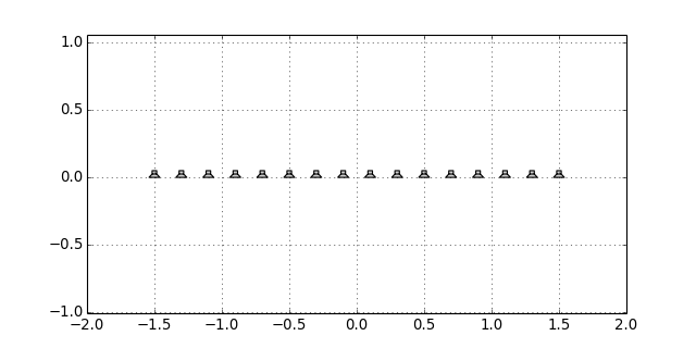
sfs.array.linear(N, spacing, center=[0, 0, 0], n0=[1, 0, 0])

Linear secondary source distribution.

Parameters:

• N (int) – Number of loudspeakers.
• spacing (float) – Distance (in metres) between loudspeakers.
• center ((3,) array_like, optional) – Coordinates of array center.
• n0 ((3,) array_like, optional) – Normal vector of array.

Returns:

• positions ((N, 3) numpy.ndarray) – Positions of secondary sources
• directions ((N, 3) numpy.ndarray) – Orientations (normal vectors) of secondary sources
• weights ((N,) numpy.ndarray) – Weights of secondary sources

Example

x0, n0, a0 = sfs.array.linear(16, 0.2, n0=[0, -1, 0])
sfs.plot.loudspeaker_2d(x0, n0, a0)
plt.axis('equal')

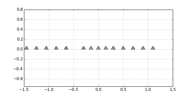
sfs.array.linear_nested(N, dx1, dx2, center=[0, 0, 0], n0=[1, 0, 0])

Nested linear secondary source distribution.

Example

x0, n0, a0 = sfs.array.linear_nested(16, 0.15, 0.2, n0=[0, -1, 0])
sfs.plot.loudspeaker_2d(x0, n0, a0)
plt.axis('equal')

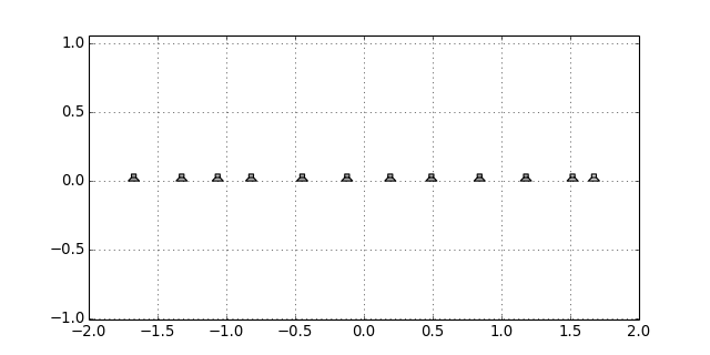
sfs.array.linear_random(N, dy1, dy2, center=[0, 0, 0], n0=[1, 0, 0])

Randomly sampled linear array.

Example

x0, n0, a0 = sfs.array.linear_random(12, 0.15, 0.4, n0=[0, -1, 0])
sfs.plot.loudspeaker_2d(x0, n0, a0)
plt.axis('equal')

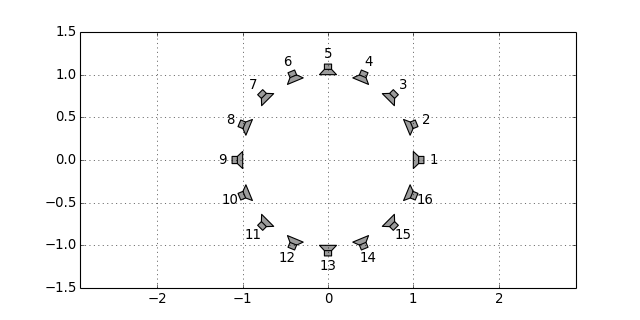
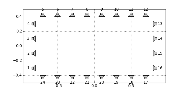
sfs.array.circular(N, R, center=[0, 0, 0])

Circular secondary source distribution parallel to the xy-plane.

Example

x0, n0, a0 = sfs.array.circular(16, 1)
sfs.plot.loudspeaker_2d(x0, n0, a0, size=0.2, show_numbers=True)
plt.axis('equal')

sfs.array.rectangular(Nx, dx, Ny, dy, center=[0, 0, 0], n0=None)

Rectangular secondary source distribution.

Example

x0, n0, a0 = sfs.array.rectangular(8, 0.2, 4, 0.2)
sfs.plot.loudspeaker_2d(x0, n0, a0, show_numbers=True)
plt.axis('equal')

sfs.array.rounded_edge(Nxy, Nr, dx, center=[0, 0, 0], n0=None)

Array along the xy-axis with rounded edge at the origin.

Parameters:

• Nxy (int) – Number of secondary sources along x- and y-axis.
• Nr (int) – Number of secondary sources in rounded edge. Radius of edge is adjusted to equdistant sampling along entire array.
• center ((3,) array_like, optional) – Position of edge.
• n0 ((3,) array_like, optional) – Normal vector of array. Default orientation is along xy-axis.

Returns:

• positions ((N, 3) numpy.ndarray) – Positions of secondary sources
• directions ((N, 3) numpy.ndarray) – Orientations (normal vectors) of secondary sources
• weights ((N,) numpy.ndarray) – Integration weights of secondary sources

Example

x0, n0, a0 = sfs.array.rounded_edge(8, 5, 0.2)
sfs.plot.loudspeaker_2d(x0, n0, a0)
plt.axis('equal')

sfs.array.planar(Ny, dy, Nz, dz, center=[0, 0, 0], n0=None)

Planar secondary source distribtion.

sfs.array.cube(Nx, dx, Ny, dy, Nz, dz, center=[0, 0, 0], n0=None)

Cube shaped secondary source distribtion.

sfs.array.sphere_load(fname, radius, center=[0, 0, 0])

Spherical secondary source distribution loaded from datafile.

ASCII Format (see MATLAB SFS Toolbox) with 4 numbers (3 position, 1 weight) per secondary source located on the unit circle.

sfs.array.load(fname, center=[0, 0, 0], n0=None)

Load secondary source positions from datafile.

Comma Seperated Values (CSV) format with 7 values (3 positions, 3 directions, 1 weight) per secondary source.

sfs.array.weights_linear(positions)

Calculate loudspeaker weights for a linear array.

The linear array has to be parallel to the y-axis.

sfs.array.weights_closed(positions)

Calculate loudspeaker weights for a simply connected array.

The weights are calculated according to the midpoint rule.

Note: The loudspeaker positions have to be ordered on the closed contour.

Tapering

Weights (tapering) for the driving function.

sfs.tapering.none(active)

No tapering window.

sfs.tapering.kaiser(active)

Kaiser tapering window.

sfs.tapering.tukey(active, alpha)

Tukey tapering window.

Monochromatic Sources

Compute the sound field generated by a sound source.

import sfs
import numpy as np
import matplotlib.pyplot as plt
plt.rcParams['figure.figsize'] = 8, 4  # inch

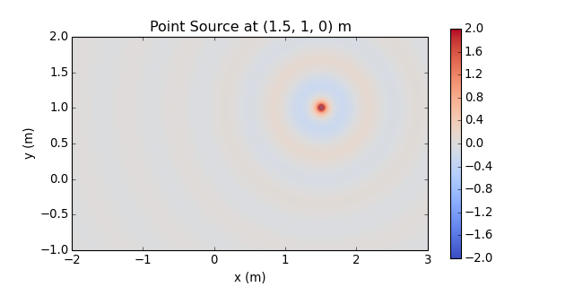
x0 = 1.5, 1, 0
f = 500  # Hz
omega = 2 * np.pi * f

grid = sfs.util.xyz_grid([-2, 3], [-1, 2], 0, spacing=0.02)

sfs.mono.source.point(omega, x0, n0, grid, c=None)

Point source.

              1  e^(-j w/c |x-x0|)
G(x-x0, w) = --- -----------------
             4pi      |x-x0|

Examples

p_point = sfs.mono.source.point(omega, x0, None, grid)
sfs.plot.soundfield(p_point, grid)
plt.title("Point Source at {} m".format(x0))

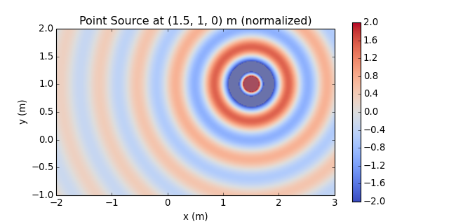
Normalization ... multiply by \(4\pi\) ...

p_point *= 4 * np.pi
sfs.plot.soundfield(p_point, grid)
plt.title("Point Source at {} m (normalized)".format(x0))

sfs.mono.source.point_modal(omega, x0, n0, grid, L, N=None, deltan=0, c=None)

Point source in a rectangular room using a modal room model.

Parameters:

• omega (float) – Frequency of source.
• x0 ((3,) array_like) – Position of source.
• n0 ((3,) array_like) – Normal vector (direction) of source (only required for compatibility).
• grid (triple of numpy.ndarray) – The grid that is used for the sound field calculations.
• L ((3,) array_like) – Dimensionons of the rectangular room.
• N ((3,) array_like or int, optional) – Combination of modal orders in the three-spatial dimensions to calculate the sound field for or maximum order for all dimensions. If not given, the maximum modal order is approximately determined and the sound field is computed up to this maximum order.
• deltan (float, optional) – Absorption coefficient of the walls.
• c (float, optional) – Speed of sound.

Returns:

numpy.ndarray – Sound pressure at positions given by grid.

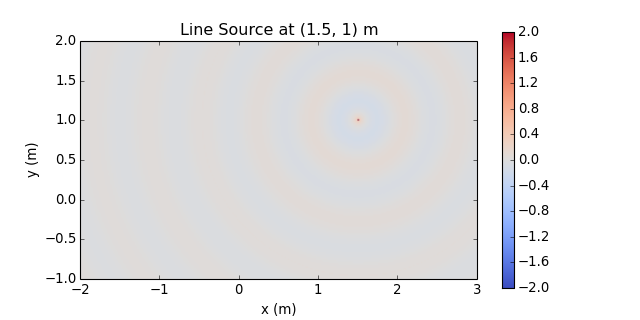
sfs.mono.source.line(omega, x0, n0, grid, c=None)

Line source parallel to the z-axis.

Note: third component of x0 is ignored.

                   (2)
G(x-x0, w) = -j/4 H0  (w/c |x-x0|)

Examples

p_line = sfs.mono.source.line(omega, x0, None, grid)
sfs.plot.soundfield(p_line, grid)
plt.title("Line Source at {} m".format(x0[:2]))

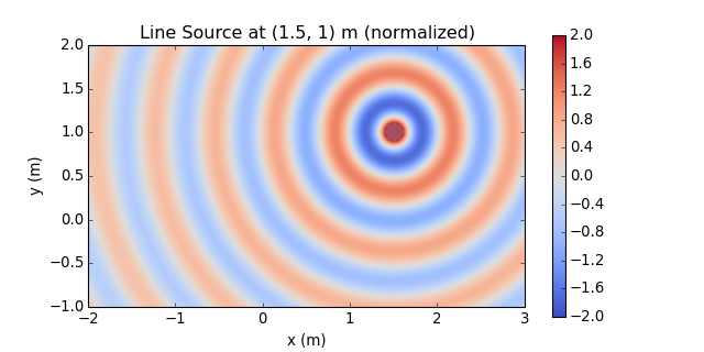
Normalization ...

p_line *= np.exp(-1j*7*np.pi/4) / np.sqrt(1/(8*np.pi*omega/sfs.defs.c))
sfs.plot.soundfield(p_line, grid)
plt.title("Line Source at {} m (normalized)".format(x0[:2]))

sfs.mono.source.line_dipole(omega, x0, n0, grid, c=None)

Line source with dipole characteristics parallel to the z-axis.

Note: third component of x0 is ignored.

                   (2)
G(x-x0, w) = jk/4 H1  (w/c |x-x0|) cos(phi)

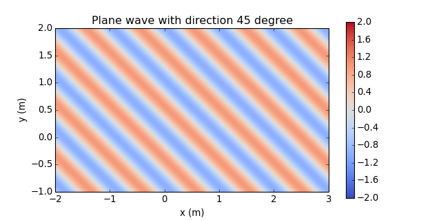
sfs.mono.source.plane(omega, x0, n0, grid, c=None)

Plane wave.

G(x, w) = e^(-i w/c n x)

Example

direction = 45  # degree
n0 = sfs.util.direction_vector(np.radians(direction))
p_plane = sfs.mono.source.plane(omega, x0, n0, grid)
sfs.plot.soundfield(p_plane, grid);
plt.title("Plane wave with direction {} degree".format(direction))

Monochromatic Driving Functions

Compute driving functions for various systems.

sfs.mono.drivingfunction.wfs_2d_line(omega, x0, n0, xs, c=None)

Line source by 2-dimensional WFS.

D(x0,k) = j k (x0-xs) n0 / |x0-xs| * H1(k |x0-xs|)

sfs.mono.drivingfunction.wfs_2d_point(omega, x0, n0, xs, c=None)

Point source by two- or three-dimensional WFS.

               (x0-xs) n0
D(x0,k) = j k ------------- e^(-j k |x0-xs|)
              |x0-xs|^(3/2)

sfs.mono.drivingfunction.wfs_25d_point(omega, x0, n0, xs, xref=[0, 0, 0], c=None, omalias=None)

Point source by 2.5-dimensional WFS.

            ____________   (x0-xs) n0
D(x0,k) = \|j k |xref-x0| ------------- e^(-j k |x0-xs|)
                          |x0-xs|^(3/2)

sfs.mono.drivingfunction.wfs_3d_point(omega, x0, n0, xs, c=None)

Point source by two- or three-dimensional WFS.

               (x0-xs) n0
D(x0,k) = j k ------------- e^(-j k |x0-xs|)
              |x0-xs|^(3/2)

sfs.mono.drivingfunction.wfs_2d_plane(omega, x0, n0, n=[0, 1, 0], c=None)

Plane wave by two- or three-dimensional WFS.

Eq.(17) from [Spors et al, 2008]:

D(x0,k) =  j k n n0  e^(-j k n x0)

sfs.mono.drivingfunction.wfs_25d_plane(omega, x0, n0, n=[0, 1, 0], xref=[0, 0, 0], c=None, omalias=None)

Plane wave by 2.5-dimensional WFS.

                 ____________
D_2.5D(x0,w) = \|j k |xref-x0| n n0 e^(-j k n x0)

sfs.mono.drivingfunction.wfs_3d_plane(omega, x0, n0, n=[0, 1, 0], c=None)

Plane wave by two- or three-dimensional WFS.

Eq.(17) from [Spors et al, 2008]:

D(x0,k) =  j k n n0  e^(-j k n x0)

sfs.mono.drivingfunction.wfs_25d_preeq(omega, omalias, c)

Preqeualization for 2.5D WFS.

sfs.mono.drivingfunction.delay_3d_plane(omega, x0, n0, n=[0, 1, 0], c=None)

Plane wave by simple delay of secondary sources.

sfs.mono.drivingfunction.source_selection_plane(n0, n)

Secondary source selection for a plane wave.

Eq.(13) from [Spors et al, 2008]

sfs.mono.drivingfunction.source_selection_point(n0, x0, xs)

Secondary source selection for a point source.

Eq.(15) from [Spors et al, 2008]

sfs.mono.drivingfunction.source_selection_all(N)

Select all secondary sources.

sfs.mono.drivingfunction.nfchoa_2d_plane(omega, x0, r0, n=[0, 1, 0], c=None)

Point source by 2.5-dimensional WFS.

sfs.mono.drivingfunction.nfchoa_25d_point(omega, x0, r0, xs, c=None)

Point source by 2.5-dimensional WFS.

                     __      (2)
              1     \       h|m| (w/c r)
D(phi0,w) = -----   /__    ------------- e^(i m (phi0-phi))
             2pi r0 m=-N..N  (2)
                            h|m| (w/c r0)

sfs.mono.drivingfunction.nfchoa_25d_plane(omega, x0, r0, n=[0, 1, 0], c=None)

Plane wave by 2.5-dimensional WFS.

                     __
                2i  \            i^|m|
D_25D(phi0,w) = --  /__    ------------------ e^(i m (phi0-phi_pw) )
                r0 m=-N..N       (2)
                            w/c h|m| (w/c r0)

sfs.mono.drivingfunction.sdm_2d_line(omega, x0, n0, xs, c=None)

Line source by two-dimensional SDM.

The secondary sources have to be located on the x-axis (y0=0). Derived from [Spors 2009, 126th AES Convention], Eq.(9), Eq.(4):

D(x0,k) =

sfs.mono.drivingfunction.sdm_2d_plane(omega, x0, n0, n=[0, 1, 0], c=None)

Plane wave by two-dimensional SDM.

The secondary sources have to be located on the x-axis (y0=0). Derived from [Ahrens 2011, Springer], Eq.(3.73), Eq.(C.5), Eq.(C.11):

D(x0,k) = kpw,y * e^(-j*kpw,x*x)

sfs.mono.drivingfunction.sdm_25d_plane(omega, x0, n0, n=[0, 1, 0], xref=[0, 0, 0], c=None)

Plane wave by 2.5-dimensional SDM.

The secondary sources have to be located on the x-axis (y0=0). Eq.(3.79) from [Ahrens 2011, Springer]:

D_2.5D(x0,w) =

sfs.mono.drivingfunction.sdm_25d_point(omega, x0, n0, xs, xref=[0, 0, 0], c=None)

Point source by 2.5-dimensional SDM.

The secondary sources have to be located on the x-axis (y0=0). Driving funcnction from [Spors 2010, 128th AES Covention], Eq.(24):

D(x0,k) =

Monochromatic Sound Fields

Computation of synthesized sound fields.

sfs.mono.synthesized.generic(omega, x0, n0, d, grid, c=None, source=<function point>)

Compute sound field for a generic driving function.

sfs.mono.synthesized.shiftphase(p, phase)

Shift pahse of a sound field.

Plotting

Plot sound fields etc.

sfs.plot.virtualsource_2d(xs, ns=None, type='point', ax=None)

Draw position/orientation of virtual source.

sfs.plot.reference_2d(xref, size=0.1, ax=None)

Draw reference/normalization point.

sfs.plot.secondarysource_2d(x0, n0, grid=None)

Simple plot of secondary source locations.

sfs.plot.loudspeaker_2d(x0, n0, a0=0.5, size=0.08, show_numbers=False, grid=None, ax=None)

Draw loudspeaker symbols at given locations and angles.

Parameters:

• x0 ((N, 3) array_like) – Loudspeaker positions.
• n0 ((N, 3) or (3,) array_like) – Normal vector(s) of loudspeakers.
• a0 (float or (N,) array_like, optional) – Weighting factor(s) of loudspeakers.
• size (float, optional) – Size of loudspeakers in metres.
• show_numbers (bool, optional) – If True, loudspeaker numbers are shown.
• grid (triple of numpy.ndarray, optional) – If specified, only loudspeakers within the grid are shown.
• ax (Axes object, optional) – The loudspeakers are plotted into this Axes object or – if not specified – into the current axes.

sfs.plot.loudspeaker_3d(x0, n0, a0=None, w=0.08, h=0.08)

Plot positions and normals of a 3D secondary source distribution.

sfs.plot.soundfield(p, grid, xnorm=None, colorbar=True, cmap='coolwarm_clip', ax=None, xlabel='x (m)', ylabel='y (m)', vmax=2.0, vmin=-2.0, **kwargs)

Two-dimensional plot of sound field.

sfs.plot.level(p, grid, xnorm=None, colorbar=True, cmap='coolwarm_clip', ax=None, xlabel='x (m)', ylabel='y (m)', vmax=3.0, vmin=-50, **kwargs)

Two-dimensional plot of level (dB) of sound field.

Utilities

Various utility functions.

sfs.util.rotation_matrix(n1, n2)

Compute rotation matrix for rotation from n1 to n2.

sfs.util.wavenumber(omega, c=None)

Compute the wavenumber for a given radial frequency.

sfs.util.direction_vector(alpha, beta=1.5707963267948966)

Compute normal vector from azimuth, colatitude.

sfs.util.sph2cart(alpha, beta, r)

Spherical to cartesian coordinates.

sfs.util.cart2sph(x, y, z)

Cartesian to spherical coordinates.

sfs.util.asarray_1d(a, **kwargs)

Squeeze the input and check if the result is one-dimensional.

Returns a converted to a numpy.ndarray and stripped of all singleton dimensions. Scalars are “upgraded” to 1D arrays. The result must have exactly one dimension. If not, an error is raised.

sfs.util.asarray_of_rows(a, **kwargs)

Convert to 2D array, turn column vector into row vector.

Returns a converted to a numpy.ndarray and stripped of all singleton dimensions. If the result has exactly one dimension, it is re-shaped into a 2D row vector.

sfs.util.asarray_of_arrays(a, **kwargs)

Convert the input to an array consisting of arrays.

A one-dimensional numpy.ndarray with dtype=object is returned, containing the elements of a as numpy.ndarray (whose dtype and other options can be specified with **kwargs).

sfs.util.strict_arange(start, stop, step=1, endpoint=False, dtype=None, **kwargs)

Like numpy.arange(), but compensating numeric errors.

Unlike numpy.arange(), but similar to numpy.linspace(), providing endpoint=True includes both endpoints.

Parameters:

• start, stop, step, dtype – See numpy.arange().

• endpoint – See numpy.linspace().

  Note

  With endpoint=True, the difference between start and end value must be an integer multiple of the corresponding spacing value!

• **kwargs – All further arguments are forwarded to numpy.isclose().

Returns:

numpy.ndarray – Array of evenly spaced values. See numpy.arange().

sfs.util.xyz_grid(x, y, z, spacing, endpoint=True, **kwargs)

Create a grid with given range and spacing.

Parameters:

• x, y, z (float or pair of float) – Inclusive range of the respective coordinate or a single value if only a slice along this dimension is needed.
• spacing (float or triple of float) – Grid spacing. If a single value is specified, it is used for all dimensions, if multiple values are given, one value is used per dimension. If a dimension (x, y or z) has only a single value, the corresponding spacing is ignored.
• endpoint (bool, optional) – If True (the default), the endpoint of each range is included in the grid. Use False to get a result similar to numpy.arange(). See strict_arange().
• **kwargs – All further arguments are forwarded to strict_arange().

Returns:

list of numpy.ndarrays – A grid that can be used for sound field calculations.

See also

strict_arange(), numpy.meshgrid()

sfs.util.normalize(p, grid, xnorm)

Normalize sound field wrt position xnorm.

sfs.util.level(p, grid, x)

Determine level at position x in the sound field p.

sfs.util.broadcast_zip(*args)

Broadcast arguments to the same shape and then use zip().

Index

Index

Version History

Version 0.1.1 (2015-10-08):

• Fix missing sfs.mono subpackage in PyPI packages

Version 0.1.0 (2015-09-22):

Initial release.