Sound Field Synthesis Toolbox for Python

Python implementation of the Sound Field Synthesis Toolbox.

Documentation:

http://sfs.rtfd.org/

Code:

http://github.com/sfstoolbox/sfs-python/

Python Package Index:

http://pypi.python.org/pypi/sfs/

License:

MIT – see the file LICENSE for details.

Requirements

Obviously, you’ll need Python. We normally use Python 3.x, but it should also work with Python 2.x. NumPy and SciPy are needed for the calculations. If you also want to plot the resulting sound fields, you’ll need matplotlib.

Instead of installing all of them separately, you should probably get a Python distribution that already includes everything, e.g. Anaconda.

Installation

Once you have installed the above-mentioned dependencies, you can use pip to download and install the latest release of the Sound Field Synthesis Toolbox with a single command:

pip install sfs --user

If you want to install it system-wide for all users (assuming you have the necessary rights), you can just drop the --user option.

To un-install, use:

pip uninstall sfs

How to Get Started

Various examples are located in the directory examples/

• sound_field_synthesis.py:

  Illustrates the general usage of the toolbox

• horizontal_plane_arrays.py:

  Computes the sound fields for various techniques, virtual sources and loudspeaker array configurations

• soundfigures.py:

  Illustrates the synthesis of sound figures with Wave Field Synthesis

Contributing

If you find errors, omissions, inconsistencies or other things that need improvement, please create an issue or a pull request at http://github.com/sfstoolbox/sfs-python/. Contributions are always welcome!

Instead of pip-installing the latest release from PyPI, you should get the newest development version from Github:

git clone https://github.com/sfstoolbox/sfs-python.git
cd sfs-python
python setup.py develop --user

This way, your installation always stays up-to-date, even if you pull new changes from the Github repository.

If you prefer, you can also replace the last command with:

pip install --user -e .

... where -e stands for --editable.

If you make changes to the documentation, you can re-create the HTML pages using Sphinx. You can install it and a few other necessary packages with:

pip install -r doc/requirements.txt --user

To create the HTML pages, use:

python setup.py build_sphinx

The generated files will be available in the directory build/sphinx/html/.

New releases are made using the following steps:

1. Bump version number in sfs/__init__.py
2. Update NEWS.rst
3. Commit those changes as “Release x.y.z”
4. Create an (annotated) tag with git tag -a x.y.z
5. Clear the dist/ directory
6. Create a source distribution with python3 setup.py sdist
7. Create a wheel distribution with python3 setup.py bdist_wheel --universal
8. Check that both files have the correct content
9. Upload them to PyPI with twine: twine upload dist/*
10. Push the commit and the tag to Github and add release notes containing a link to PyPI and the bullet points from NEWS.rst
11. Check that the new release was built correctly on RTD, delete the “stable” version and select the new release as default version

API Documentation

Loudspeaker Arrays

Compute positions of various secondary source distributions.

import sfs
import matplotlib.pyplot as plt
plt.rcParams['figure.figsize'] = 8, 4.5  # inch
plt.rcParams['axes.grid'] = True

class sfs.array.ArrayData

Named tuple returned by array functions.

See collections.namedtuple.

x

(N, 3) numpy.ndarray – Positions of secondary sources

n

(N, 3) numpy.ndarray – Orientations (normal vectors) of secondary sources

a

(N,) numpy.ndarray – Weights of secondary sources

take(indices)

Return a sub-array given by indices.

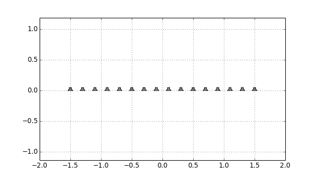
sfs.array.linear(N, spacing, center=[0, 0, 0], orientation=[1, 0, 0])

Linear secondary source distribution.

Parameters:

• N (int) – Number of secondary sources.
• spacing (float) – Distance (in metres) between secondary sources.
• center ((3,) array_like, optional) – Coordinates of array center.
• orientation ((3,) array_like, optional) – Orientation of the array. By default, the loudspeakers have their main axis pointing into positive x-direction.

Returns:

ArrayData – Positions, orientations and weights of secondary sources. See ArrayData.

Examples

x0, n0, a0 = sfs.array.linear(16, 0.2, orientation=[0, -1, 0])
sfs.plot.loudspeaker_2d(x0, n0, a0)
plt.axis('equal')

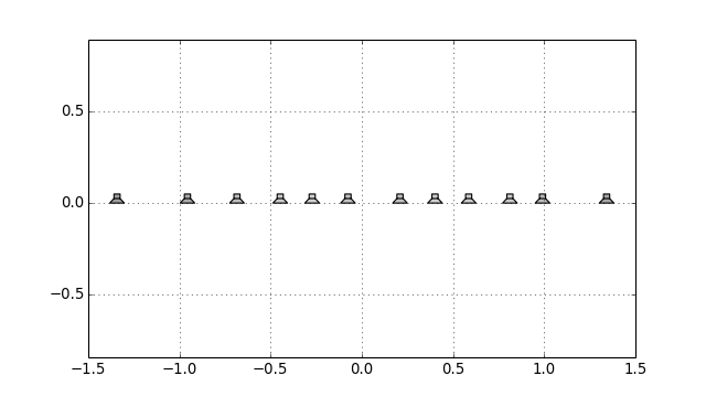
sfs.array.linear_diff(distances, center=[0, 0, 0], orientation=[1, 0, 0])

Linear secondary source distribution from a list of distances.

Parameters:

• distances ((N-1,) array_like) – Sequence of secondary sources distances in metres.
• center, orientation – See linear()

Returns:

ArrayData – Positions, orientations and weights of secondary sources. See ArrayData.

Examples

x0, n0, a0 = sfs.array.linear_diff(4 * [0.3] + 6 * [0.15] + 4 * [0.3],
                                   orientation=[0, -1, 0])
sfs.plot.loudspeaker_2d(x0, n0, a0)
plt.axis('equal')

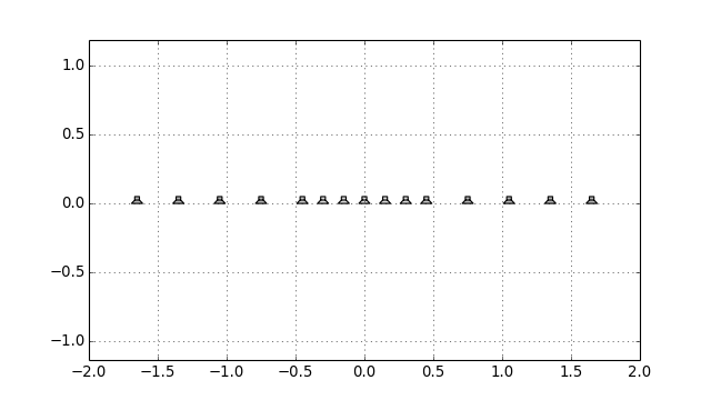
sfs.array.linear_random(N, min_spacing, max_spacing, center=[0, 0, 0], orientation=[1, 0, 0], seed=None)

Randomly sampled linear array.

Parameters:

• N (int) – Number of secondary sources.
• min_spacing, max_spacing (float) – Minimal and maximal distance (in metres) between secondary sources.
• center, orientation – See linear()
• seed ({None, int, array_like}, optional) – Random seed. See numpy.random.RandomState.

Returns:

ArrayData – Positions, orientations and weights of secondary sources. See ArrayData.

Examples

x0, n0, a0 = sfs.array.linear_random(12, 0.15, 0.4, orientation=[0, -1, 0])
sfs.plot.loudspeaker_2d(x0, n0, a0)
plt.axis('equal')

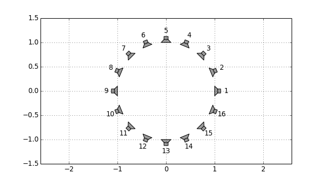
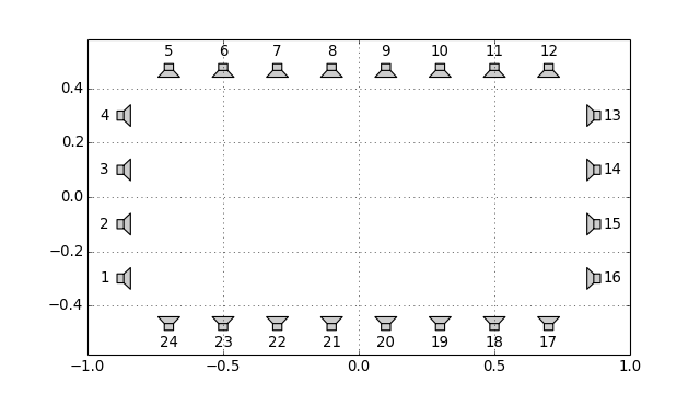
sfs.array.circular(N, R, center=[0, 0, 0])

Circular secondary source distribution parallel to the xy-plane.

Parameters:

• N (int) – Number of secondary sources.
• R (float) – Radius in metres.
• center – See linear().

Returns:

ArrayData – Positions, orientations and weights of secondary sources. See ArrayData.

Examples

x0, n0, a0 = sfs.array.circular(16, 1)
sfs.plot.loudspeaker_2d(x0, n0, a0, size=0.2, show_numbers=True)
plt.axis('equal')

sfs.array.rectangular(N, spacing, center=[0, 0, 0], orientation=[1, 0, 0])

Rectangular secondary source distribution.

Parameters:

• N (int or pair of int) – Number of secondary sources on each side of the rectangle. If a pair of numbers is given, the first one specifies the first and third segment, the second number specifies the second and fourth segment.
• spacing (float) – Distance (in metres) between secondary sources.
• center, orientation – See linear(). The orientation corresponds to the first linear segment.

Returns:

ArrayData – Positions, orientations and weights of secondary sources. See ArrayData.

Examples

x0, n0, a0 = sfs.array.rectangular((4, 8), 0.2)
sfs.plot.loudspeaker_2d(x0, n0, a0, show_numbers=True)
plt.axis('equal')

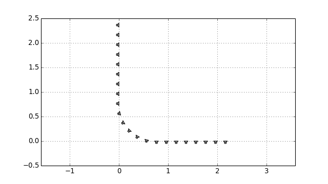
sfs.array.rounded_edge(Nxy, Nr, dx, center=[0, 0, 0], orientation=[1, 0, 0])

Array along the xy-axis with rounded edge at the origin.

Parameters:

• Nxy (int) – Number of secondary sources along x- and y-axis.
• Nr (int) – Number of secondary sources in rounded edge. Radius of edge is adjusted to equdistant sampling along entire array.
• center ((3,) array_like, optional) – Position of edge.
• orientation ((3,) array_like, optional) – Normal vector of array. Default orientation is along xy-axis.

Returns:

ArrayData – Positions, orientations and weights of secondary sources. See ArrayData.

Examples

x0, n0, a0 = sfs.array.rounded_edge(8, 5, 0.2)
sfs.plot.loudspeaker_2d(x0, n0, a0)
plt.axis('equal')

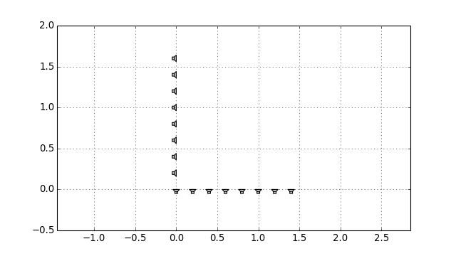
sfs.array.edge(Nxy, dx, center=[0, 0, 0], orientation=[1, 0, 0])

Array along the xy-axis with edge at the origin.

Parameters:

• Nxy (int) – Number of secondary sources along x- and y-axis.
• center ((3,) array_like, optional) – Position of edge.
• orientation ((3,) array_like, optional) – Normal vector of array. Default orientation is along xy-axis.

Returns:

ArrayData – Positions, orientations and weights of secondary sources. See ArrayData.

Examples

x0, n0, a0 = sfs.array.edge(8, 0.2)
sfs.plot.loudspeaker_2d(x0, n0, a0)
plt.axis('equal')

sfs.array.planar(N, spacing, center=[0, 0, 0], orientation=[1, 0, 0])

Planar secondary source distribtion.

Parameters:

• N (int or pair of int) – Number of secondary sources along each edge. If a pair of numbers is given, the first one specifies the number on the horizontal edge, the second one specifies the number on the vertical edge.
• spacing (float) – Distance (in metres) between secondary sources.
• center, orientation – See linear().

Returns:

ArrayData – Positions, orientations and weights of secondary sources. See ArrayData.

sfs.array.cube(N, spacing, center=[0, 0, 0], orientation=[1, 0, 0])

Cube-shaped secondary source distribtion.

Parameters:

• N (int or triple of int) – Number of secondary sources along each edge. If a triple of numbers is given, the first two specify the edges like in rectangular(), the last one specifies the vertical edge.
• spacing (float) – Distance (in metres) between secondary sources.
• center, orientation – See linear(). The orientation corresponds to the first planar segment.

Returns:

ArrayData – Positions, orientations and weights of secondary sources. See ArrayData.

sfs.array.sphere_load(fname, radius, center=[0, 0, 0])

Spherical secondary source distribution loaded from datafile.

ASCII Format (see MATLAB SFS Toolbox) with 4 numbers (3 position, 1 weight) per secondary source located on the unit circle.

Returns:ArrayData – Positions, orientations and weights of secondary sources. See ArrayData.

sfs.array.load(fname, center=[0, 0, 0], orientation=[1, 0, 0])

Load secondary source positions from datafile.

Comma Seperated Values (CSV) format with 7 values (3 positions, 3 normal vectors, 1 weight) per secondary source.

Returns:ArrayData – Positions, orientations and weights of secondary sources. See ArrayData.

sfs.array.weights_midpoint(positions, closed)

Calculate loudspeaker weights for a simply connected array.

The weights are calculated according to the midpoint rule.

Parameters:

• positions ((N, 3) array_like) – Sequence of secondary source positions.

  Note

  The loudspeaker positions have to be ordered on the contour!

• closed (bool) – True if the loudspeaker contour is closed.

Returns:

(N,) numpy.ndarray – Weights of secondary sources.

sfs.array.concatenate(*arrays)

Concatenate ArrayData objects.

Tapering

Weights (tapering) for the driving function.

sfs.tapering.none(active)

No tapering window.

sfs.tapering.kaiser(active)

Kaiser tapering window.

sfs.tapering.tukey(active, alpha)

Tukey tapering window.

Monochromatic Sources

Compute the sound field generated by a sound source.

import sfs
import numpy as np
import matplotlib.pyplot as plt
plt.rcParams['figure.figsize'] = 8, 4.5  # inch

x0 = 1.5, 1, 0
f = 500  # Hz
omega = 2 * np.pi * f

normalization_point = 4 * np.pi
normalization_line = \
    np.sqrt(8 * np.pi * omega / sfs.defs.c) * np.exp(1j * np.pi / 4)

grid = sfs.util.xyz_grid([-2, 3], [-1, 2], 0, spacing=0.02)

# Grid for vector fields:
vgrid = sfs.util.xyz_grid([-2, 3], [-1, 2], 0, spacing=0.1)

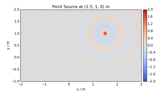
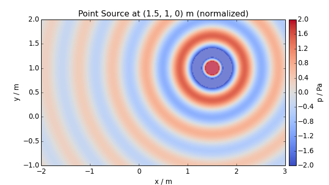
sfs.mono.source.point(omega, x0, n0, grid, c=None)

Point source.

Notes

              1  e^(-j w/c |x-x0|)
G(x-x0, w) = --- -----------------
             4pi      |x-x0|

Examples

p = sfs.mono.source.point(omega, x0, None, grid)
sfs.plot.soundfield(p, grid)
plt.title("Point Source at {} m".format(x0))

Normalization ...

sfs.plot.soundfield(p * normalization_point, grid,
                    colorbar_kwargs=dict(label="p / Pa"))
plt.title("Point Source at {} m (normalized)".format(x0))

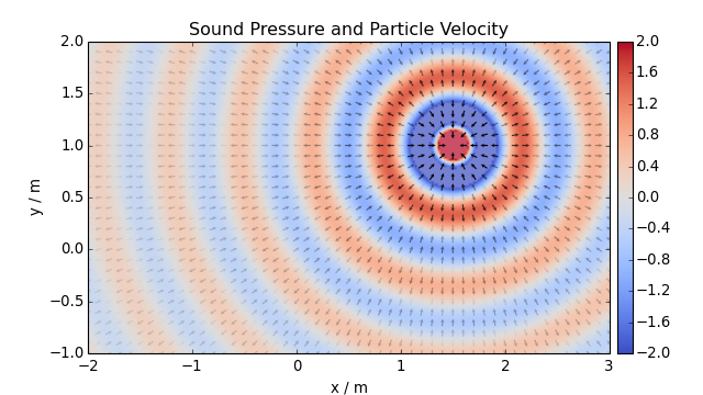
sfs.mono.source.point_velocity(omega, x0, n0, grid, c=None)

Velocity of a point source.

Returns:XyzComponents – Particle velocity at positions given by grid. See sfs.util.XyzComponents.

Examples

The particle velocity can be plotted on top of the sound pressure:

v = sfs.mono.source.point_velocity(omega, x0, None, vgrid)
sfs.plot.soundfield(p * normalization_point, grid)
sfs.plot.vectors(v * normalization_point, vgrid)
plt.title("Sound Pressure and Particle Velocity")

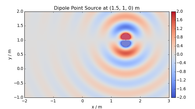
sfs.mono.source.point_dipole(omega, x0, n0, grid, c=None)

Point source with dipole characteristics.

Parameters:

• omega (float) – Frequency of source.
• x0 ((3,) array_like) – Position of source.
• n0 ((3,) array_like) – Normal vector (direction) of dipole.
• grid (triple of array_like) – The grid that is used for the sound field calculations. See sfs.util.xyz_grid().
• c (float, optional) – Speed of sound.

Returns:

numpy.ndarray – Sound pressure at positions given by grid.

Notes

 d                1   / iw       1    \   (x-x0) n0
---- G(x-x0,w) = --- | ----- + ------- | ----------- e^(-i w/c |x-x0|)
d ns             4pi  \  c     |x-x0| /   |x-x0|^2

Examples

n0 = 0, 1, 0
p = sfs.mono.source.point_dipole(omega, x0, n0, grid)
sfs.plot.soundfield(p, grid)
plt.title("Dipole Point Source at {} m".format(x0))

sfs.mono.source.point_modal(omega, x0, n0, grid, L, N=None, deltan=0, c=None)

Point source in a rectangular room using a modal room model.

Parameters:

• omega (float) – Frequency of source.
• x0 ((3,) array_like) – Position of source.
• n0 ((3,) array_like) – Normal vector (direction) of source (only required for compatibility).
• grid (triple of array_like) – The grid that is used for the sound field calculations. See sfs.util.xyz_grid().
• L ((3,) array_like) – Dimensionons of the rectangular room.
• N ((3,) array_like or int, optional) – Combination of modal orders in the three-spatial dimensions to calculate the sound field for or maximum order for all dimensions. If not given, the maximum modal order is approximately determined and the sound field is computed up to this maximum order.
• deltan (float, optional) – Absorption coefficient of the walls.
• c (float, optional) – Speed of sound.

Returns:

numpy.ndarray – Sound pressure at positions given by grid.

sfs.mono.source.point_modal_velocity(omega, x0, n0, grid, L, N=None, deltan=0, c=None)

Velocity of point source in a rectangular room using a modal room model.

Parameters:

• omega (float) – Frequency of source.
• x0 ((3,) array_like) – Position of source.
• n0 ((3,) array_like) – Normal vector (direction) of source (only required for compatibility).
• grid (triple of array_like) – The grid that is used for the sound field calculations. See sfs.util.xyz_grid().
• L ((3,) array_like) – Dimensionons of the rectangular room.
• N ((3,) array_like or int, optional) – Combination of modal orders in the three-spatial dimensions to calculate the sound field for or maximum order for all dimensions. If not given, the maximum modal order is approximately determined and the sound field is computed up to this maximum order.
• deltan (float, optional) – Absorption coefficient of the walls.
• c (float, optional) – Speed of sound.

Returns:

XyzComponents – Particle velocity at positions given by grid. See sfs.util.XyzComponents.

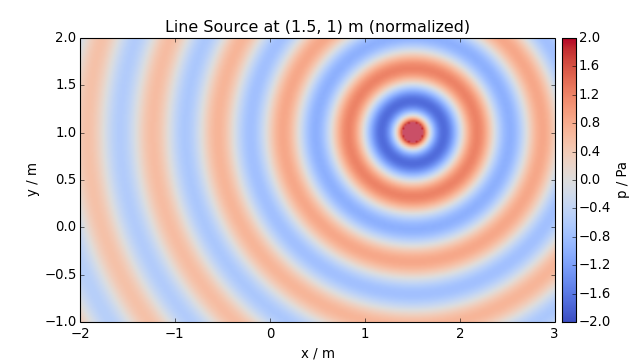
sfs.mono.source.line(omega, x0, n0, grid, c=None)

Line source parallel to the z-axis.

Note: third component of x0 is ignored.

Notes

                   (2)
G(x-x0, w) = -j/4 H0  (w/c |x-x0|)

Examples

p = sfs.mono.source.line(omega, x0, None, grid)
sfs.plot.soundfield(p, grid)
plt.title("Line Source at {} m".format(x0[:2]))

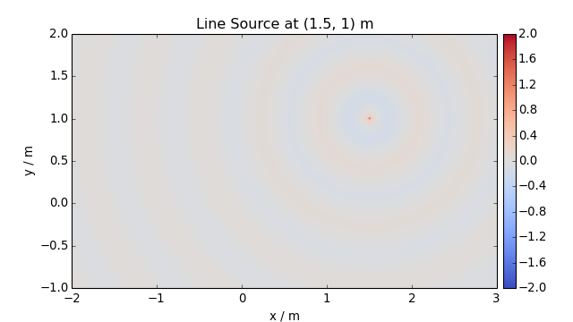
Normalization ...

sfs.plot.soundfield(p * normalization_line, grid,
                    colorbar_kwargs=dict(label="p / Pa"))
plt.title("Line Source at {} m (normalized)".format(x0[:2]))

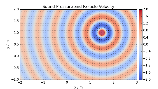
sfs.mono.source.line_velocity(omega, x0, n0, grid, c=None)

Velocity of line source parallel to the z-axis.

Returns:XyzComponents – Particle velocity at positions given by grid. See sfs.util.XyzComponents.

Examples

The particle velocity can be plotted on top of the sound pressure:

v = sfs.mono.source.line_velocity(omega, x0, None, vgrid)
sfs.plot.soundfield(p * normalization_line, grid)
sfs.plot.vectors(v * normalization_line, vgrid)
plt.title("Sound Pressure and Particle Velocity")

sfs.mono.source.line_dipole(omega, x0, n0, grid, c=None)

Line source with dipole characteristics parallel to the z-axis.

Note: third component of x0 is ignored.

Notes

                   (2)
G(x-x0, w) = jk/4 H1  (w/c |x-x0|) cos(phi)

sfs.mono.source.line_dirichlet_edge(omega, x0, grid, alpha=4.71238898038469, Nc=None, c=None)

Sound field of an line source scattered at an edge with Dirichlet

boundary conditions.

[Michael Möser, Technische Akustik, 2012, Springer, eq.(10.18/19)]

Parameters:

• omega (float) – Angular frequency.
• x0 ((3,) array_like) – Position of line source.
• XyzComponents – A grid that is used for calculations of the sound field.
• alpha (float, optional) – Outer angle of edge.
• Nc (int, optional) – Number of elements for series expansion of driving function. Estimated if not given.
• c (float, optional) – Speed of sound

Returns:

() numpy.ndarray – Complex pressure at grid positions.

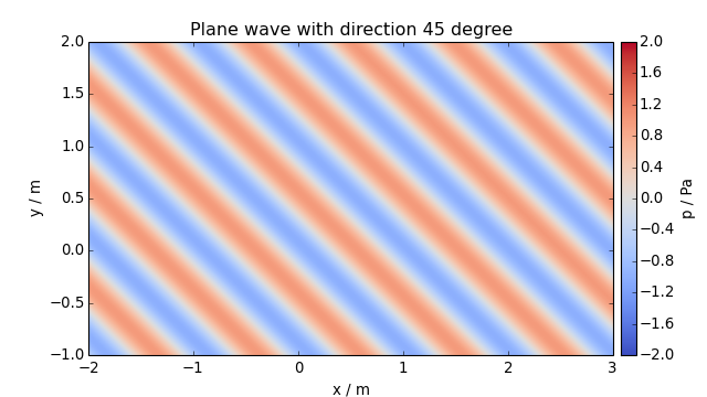
sfs.mono.source.plane(omega, x0, n0, grid, c=None)

Plane wave.

Notes

G(x, w) = e^(-i w/c n x)

Examples

direction = 45  # degree
n0 = sfs.util.direction_vector(np.radians(direction))
p = sfs.mono.source.plane(omega, x0, n0, grid)
sfs.plot.soundfield(p, grid, colorbar_kwargs=dict(label="p / Pa"))
plt.title("Plane wave with direction {} degree".format(direction))

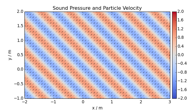
sfs.mono.source.plane_velocity(omega, x0, n0, grid, c=None)

Velocity of a plane wave.

Notes

V(x, w) = 1/(rho c) e^(-i w/c n x) n

Returns:XyzComponents – Particle velocity at positions given by grid. See sfs.util.XyzComponents.

Examples

The particle velocity can be plotted on top of the sound pressure:

v = sfs.mono.source.plane_velocity(omega, x0, n0, vgrid)
sfs.plot.soundfield(p, grid)
sfs.plot.vectors(v, vgrid)
plt.title("Sound Pressure and Particle Velocity")

Monochromatic Driving Functions

Compute driving functions for various systems.

sfs.mono.drivingfunction.wfs_2d_line(omega, x0, n0, xs, c=None)

Line source by 2-dimensional WFS.

D(x0,k) = j/2 k (x0-xs) n0 / |x0-xs| * H1(k |x0-xs|)

sfs.mono.drivingfunction.wfs_2d_point(omega, x0, n0, xs, c=None)

Point source by two- or three-dimensional WFS.

               (x0-xs) n0
D(x0,k) = j k ------------- e^(-j k |x0-xs|)
              |x0-xs|^(3/2)

sfs.mono.drivingfunction.wfs_25d_point(omega, x0, n0, xs, xref=[0, 0, 0], c=None, omalias=None)

Point source by 2.5-dimensional WFS.

            ____________   (x0-xs) n0
D(x0,k) = \|j k |xref-x0| ------------- e^(-j k |x0-xs|)
                          |x0-xs|^(3/2)

sfs.mono.drivingfunction.wfs_3d_point(omega, x0, n0, xs, c=None)

Point source by two- or three-dimensional WFS.

               (x0-xs) n0
D(x0,k) = j k ------------- e^(-j k |x0-xs|)
              |x0-xs|^(3/2)

sfs.mono.drivingfunction.wfs_2d_plane(omega, x0, n0, n=[0, 1, 0], c=None)

Plane wave by two- or three-dimensional WFS.

Eq.(17) from [Spors et al, 2008]:

D(x0,k) =  j k n n0  e^(-j k n x0)

sfs.mono.drivingfunction.wfs_25d_plane(omega, x0, n0, n=[0, 1, 0], xref=[0, 0, 0], c=None, omalias=None)

Plane wave by 2.5-dimensional WFS.

                 ____________
D_2.5D(x0,w) = \|j k |xref-x0| n n0 e^(-j k n x0)

sfs.mono.drivingfunction.wfs_3d_plane(omega, x0, n0, n=[0, 1, 0], c=None)

Plane wave by two- or three-dimensional WFS.

Eq.(17) from [Spors et al, 2008]:

D(x0,k) =  j k n n0  e^(-j k n x0)

sfs.mono.drivingfunction.wfs_2d_focused(omega, x0, n0, xs, c=None)

Focused source by two- or three-dimensional WFS.

               (x0-xs) n0
D(x0,k) = j k ------------- e^(j k |x0-xs|)
              |x0-xs|^(3/2)

sfs.mono.drivingfunction.wfs_25d_focused(omega, x0, n0, xs, xref=[0, 0, 0], c=None, omalias=None)

Focused source by 2.5-dimensional WFS.

            ____________   (x0-xs) n0
D(x0,w) = \|j k |xref-x0| ------------- e^(j k |x0-xs|)
                          |x0-xs|^(3/2)

sfs.mono.drivingfunction.wfs_3d_focused(omega, x0, n0, xs, c=None)

Focused source by two- or three-dimensional WFS.

               (x0-xs) n0
D(x0,k) = j k ------------- e^(j k |x0-xs|)
              |x0-xs|^(3/2)

sfs.mono.drivingfunction.wfs_25d_preeq(omega, omalias, c)

Preqeualization for 2.5D WFS.

sfs.mono.drivingfunction.delay_3d_plane(omega, x0, n0, n=[0, 1, 0], c=None)

Plane wave by simple delay of secondary sources.

sfs.mono.drivingfunction.source_selection_plane(n0, n)

Secondary source selection for a plane wave.

Eq.(13) from [Spors et al, 2008]

sfs.mono.drivingfunction.source_selection_point(n0, x0, xs)

Secondary source selection for a point source.

Eq.(15) from [Spors et al, 2008]

sfs.mono.drivingfunction.source_selection_line(n0, x0, xs)

Secondary source selection for a line source.

compare Eq.(15) from [Spors et al, 2008]

sfs.mono.drivingfunction.source_selection_focused(ns, x0, xs)

Secondary source selection for a focused source.

Eq.(2.78) from [Wierstorf, 2014]

sfs.mono.drivingfunction.source_selection_all(N)

Select all secondary sources.

sfs.mono.drivingfunction.nfchoa_2d_plane(omega, x0, r0, n=[0, 1, 0], c=None)

Plane wave by two-dimensional NFC-HOA.

                       __
               2i     \        i^-m
D(phi0,w) = - -----   /__   ----------  e^(i m (phi0-phi_pw))
              pi r0 m=-N..N  (2)
                            Hm  (w/c r0)

sfs.mono.drivingfunction.nfchoa_25d_point(omega, x0, r0, xs, c=None)

Point source by 2.5-dimensional NFC-HOA.

                     __      (2)
              1     \       h|m| (w/c r)
D(phi0,w) = -----   /__    ------------- e^(i m (phi0-phi))
             2pi r0 m=-N..N  (2)
                            h|m| (w/c r0)

sfs.mono.drivingfunction.nfchoa_25d_plane(omega, x0, r0, n=[0, 1, 0], c=None)

Plane wave by 2.5-dimensional NFC-HOA.

                     __
                2i  \            i^|m|
D_25D(phi0,w) = --  /__    ------------------ e^(i m (phi0-phi_pw) )
                r0 m=-N..N       (2)
                            w/c h|m| (w/c r0)

sfs.mono.drivingfunction.sdm_2d_line(omega, x0, n0, xs, c=None)

Line source by two-dimensional SDM.

The secondary sources have to be located on the x-axis (y0=0). Derived from [Spors 2009, 126th AES Convention], Eq.(9), Eq.(4):

D(x0,k) =

sfs.mono.drivingfunction.sdm_2d_plane(omega, x0, n0, n=[0, 1, 0], c=None)

Plane wave by two-dimensional SDM.

The secondary sources have to be located on the x-axis (y0=0). Derived from [Ahrens 2011, Springer], Eq.(3.73), Eq.(C.5), Eq.(C.11):

D(x0,k) = kpw,y * e^(-j*kpw,x*x)

sfs.mono.drivingfunction.sdm_25d_plane(omega, x0, n0, n=[0, 1, 0], xref=[0, 0, 0], c=None)

Plane wave by 2.5-dimensional SDM.

The secondary sources have to be located on the x-axis (y0=0). Eq.(3.79) from [Ahrens 2011, Springer]:

D_2.5D(x0,w) =

sfs.mono.drivingfunction.sdm_25d_point(omega, x0, n0, xs, xref=[0, 0, 0], c=None)

Point source by 2.5-dimensional SDM.

The secondary sources have to be located on the x-axis (y0=0). Driving funcnction from [Spors 2010, 128th AES Covention], Eq.(24):

D(x0,k) =

sfs.mono.drivingfunction.esa_edge_2d_plane(omega, x0, n=[0, 1, 0], alpha=4.71238898038469, Nc=None, c=None)

Plane wave by two-dimensional ESA for an edge-shaped secondary source

distribution consisting of monopole line sources.

One leg of the secondary sources has to be located on the x-axis (y0=0), the edge at the origin.

Derived from [Spors 2016, DAGA]

Parameters:

• omega (float) – Angular frequency.
• x0 (int(N, 3) array_like) – Sequence of secondary source positions.
• n ((3,) array_like, optional) – Normal vector of synthesized plane wave.
• alpha (float, optional) – Outer angle of edge.
• Nc (int, optional) – Number of elements for series expansion of driving function. Estimated if not given.
• c (float, optional) – Speed of sound

Returns:

(N,) numpy.ndarray – Complex weights of secondary sources.

sfs.mono.drivingfunction.esa_edge_dipole_2d_plane(omega, x0, n=[0, 1, 0], alpha=4.71238898038469, Nc=None, c=None)

Plane wave by two-dimensional ESA for an edge-shaped secondary source

distribution consisting of dipole line sources.

One leg of the secondary sources has to be located on the x-axis (y0=0), the edge at the origin.

Derived from [Spors 2016, DAGA]

Parameters:

• omega (float) – Angular frequency.
• x0 (int(N, 3) array_like) – Sequence of secondary source positions.
• n ((3,) array_like, optional) – Normal vector of synthesized plane wave.
• alpha (float, optional) – Outer angle of edge.
• Nc (int, optional) – Number of elements for series expansion of driving function. Estimated if not given.
• c (float, optional) – Speed of sound

Returns:

(N,) numpy.ndarray – Complex weights of secondary sources.

sfs.mono.drivingfunction.esa_edge_2d_line(omega, x0, xs, alpha=4.71238898038469, Nc=None, c=None)

Line source by two-dimensional ESA for an edge-shaped secondary source

distribution constisting of monopole line sources.

One leg of the secondary sources have to be located on the x-axis (y0=0), the edge at the origin.

Derived from [Spors 2016, DAGA]

Parameters:

• omega (float) – Angular frequency.
• x0 (int(N, 3) array_like) – Sequence of secondary source positions.
• xs ((3,) array_like) – Position of synthesized line source.
• alpha (float, optional) – Outer angle of edge.
• Nc (int, optional) – Number of elements for series expansion of driving function. Estimated if not given.
• c (float, optional) – Speed of sound

Returns:

(N,) numpy.ndarray – Complex weights of secondary sources.

sfs.mono.drivingfunction.esa_edge_25d_point(omega, x0, xs, xref=[2, -2, 0], alpha=4.71238898038469, Nc=None, c=None)

Point source by 2.5-dimensional ESA for an edge-shaped secondary source

distribution constisting of monopole line sources.

One leg of the secondary sources have to be located on the x-axis (y0=0), the edge at the origin.

Derived from [Spors 2016, DAGA]

Parameters:

• omega (float) – Angular frequency.
• x0 (int(N, 3) array_like) – Sequence of secondary source positions.
• xs ((3,) array_like) – Position of synthesized line source.
• xref ((3,) array_like or float) – Reference position or reference distance
• alpha (float, optional) – Outer angle of edge.
• Nc (int, optional) – Number of elements for series expansion of driving function. Estimated if not given.
• c (float, optional) – Speed of sound

Returns:

(N,) numpy.ndarray – Complex weights of secondary sources.

sfs.mono.drivingfunction.esa_edge_dipole_2d_line(omega, x0, xs, alpha=4.71238898038469, Nc=None, c=None)

Line source by two-dimensional ESA for an edge-shaped secondary source

distribution constisting of dipole line sources.

One leg of the secondary sources have to be located on the x-axis (y0=0), the edge at the origin.

Derived from [Spors 2016, DAGA]

Parameters:

• omega (float) – Angular frequency.
• x0 ((N, 3) array_like) – Sequence of secondary source positions.
• xs ((3,) array_like) – Position of synthesized line source.
• alpha (float, optional) – Outer angle of edge.
• Nc (int, optional) – Number of elements for series expansion of driving function. Estimated if not given.
• c (float, optional) – Speed of sound

Returns:

(N,) numpy.ndarray – Complex weights of secondary sources.

Monochromatic Sound Fields

Computation of synthesized sound fields.

sfs.mono.synthesized.generic(omega, x0, n0, d, grid, c=None, source=<function point>)

Compute sound field for a generic driving function.

sfs.mono.synthesized.shiftphase(p, phase)

Shift phase of a sound field.

Plotting

Plot sound fields etc.

sfs.plot.virtualsource_2d(xs, ns=None, type='point', ax=None)

Draw position/orientation of virtual source.

sfs.plot.reference_2d(xref, size=0.1, ax=None)

Draw reference/normalization point.

sfs.plot.secondarysource_2d(x0, n0, grid=None)

Simple plot of secondary source locations.

sfs.plot.loudspeaker_2d(x0, n0, a0=0.5, size=0.08, show_numbers=False, grid=None, ax=None)

Draw loudspeaker symbols at given locations and angles.

Parameters:

• x0 ((N, 3) array_like) – Loudspeaker positions.
• n0 ((N, 3) or (3,) array_like) – Normal vector(s) of loudspeakers.
• a0 (float or (N,) array_like, optional) – Weighting factor(s) of loudspeakers.
• size (float, optional) – Size of loudspeakers in metres.
• show_numbers (bool, optional) – If True, loudspeaker numbers are shown.
• grid (triple of numpy.ndarray, optional) – If specified, only loudspeakers within the grid are shown.
• ax (Axes object, optional) – The loudspeakers are plotted into this Axes object or – if not specified – into the current axes.

sfs.plot.loudspeaker_3d(x0, n0, a0=None, w=0.08, h=0.08)

Plot positions and normals of a 3D secondary source distribution.

sfs.plot.soundfield(p, grid, xnorm=None, cmap='coolwarm_clip', vmin=-2.0, vmax=2.0, xlabel=None, ylabel=None, colorbar=True, colorbar_kwargs={}, ax=None, **kwargs)

Two-dimensional plot of sound field.

Parameters:

• p (array_like) – Sound pressure values (or any other scalar quantity if you like). If the values are complex, the imaginary part is ignored. Typically, p is two-dimensional with a shape of (Ny, Nx), (Nz, Nx) or (Nz, Ny). This is the case if sfs.util.xyz_grid() was used with a single number for z, y or x, respectively. However, p can also be three-dimensional with a shape of (Ny, Nx, 1), (1, Nx, Nz) or (Ny, 1, Nz). This is the case if numpy.meshgrid() was used with a scalar for z, y or x, respectively (and of course with the default indexing='xy').

  Note

  If you want to plot a single slice of a pre-computed “full” 3D sound field, make sure that the slice still has three dimensions (including one singleton dimension). This way, you can use the original grid of the full volume without changes. This works because the grid component corresponding to the singleton dimension is simply ignored.

• grid (triple or pair of numpy.ndarray) – The grid that was used to calculate p, see sfs.util.xyz_grid(). If p is two-dimensional, but grid has 3 components, one of them must be scalar.

• xnorm (array_like, optional) – Coordinates of a point to which the sound field should be normalized before plotting. If not specified, no normalization is used. See sfs.util.normalize().

Returns:

AxesImage – See matplotlib.pyplot.imshow().

Other Parameters:  

• xlabel, ylabel (str) – Overwrite default x/y labels. Use xlabel='' and ylabel='' to remove x/y labels. The labels can be changed afterwards with matplotlib.pyplot.xlabel() and matplotlib.pyplot.ylabel().
• colorbar (bool, optional) – If False, no colorbar is created.
• colorbar_kwargs (dict, optional) – Further colorbar arguments, see add_colorbar().
• ax (Axes, optional) – If given, the plot is created on ax instead of the current axis (see matplotlib.pyplot.gca()).
• cmap, vmin, vmax, **kwargs – All further parameters are forwarded to matplotlib.pyplot.imshow().

See also

sfs.plot.level()

sfs.plot.level(p, grid, xnorm=None, power=False, cmap=None, vmax=3, vmin=-50, **kwargs)

Two-dimensional plot of level (dB) of sound field.

Takes the same parameters as sfs.plot.soundfield().

Other Parameters:  power (bool, optional) – See sfs.util.db().

sfs.plot.particles(x, trim=None, ax=None, xlabel='x (m)', ylabel='y (m)', edgecolor='', **kwargs)

Plot particle positions as scatter plot

sfs.plot.vectors(v, grid, cmap='blacktransparent', headlength=3, headaxislength=2.5, ax=None, clim=None, **kwargs)

Plot a vector field in the xy plane.

Parameters:

• v (triple or pair of array_like) – x, y and optionally z components of vector field. The z components are ignored. If the values are complex, the imaginary parts are ignored.
• grid (triple or pair of array_like) – The grid that was used to calculate v, see sfs.util.xyz_grid(). Any z components are ignored.

Returns:

Quiver – See matplotlib.pyplot.quiver().

Other Parameters:  

• ax (Axes, optional) – If given, the plot is created on ax instead of the current axis (see matplotlib.pyplot.gca()).
• clim (pair of float, optional) – Limits for the scaling of arrow colors. See matplotlib.pyplot.quiver().
• cmap, headlength, headaxislength, **kwargs – All further parameters are forwarded to matplotlib.pyplot.quiver().

sfs.plot.add_colorbar(im, aspect=20, pad=0.5, **kwargs)

Add a vertical color bar to a plot.

Parameters:

• im (ScalarMappable) – The output of sfs.plot.soundfield(), sfs.plot.level() or any other matplotlib.cm.ScalarMappable.

• aspect (float, optional) – Aspect ratio of the colorbar. Strictly speaking, since the colorbar is vertical, it’s actually the inverse of the aspect ratio.

• pad (float, optional) – Space between image plot and colorbar, as a fraction of the width of the colorbar.

  Note

  The pad argument of matplotlib.figure.Figure.colorbar() has a slightly different meaning (“fraction of original axes”)!

• **kwargs – All further arguments are forwarded to matplotlib.figure.Figure.colorbar().

See also

matplotlib.pyplot.colorbar()

Utilities

Various utility functions.

sfs.util.rotation_matrix(n1, n2)

Compute rotation matrix for rotation from n1 to n2.

Parameters:n1, n2 ((3,) array_like) – Two vectors. They don’t have to be normalized. Returns:(3, 3) numpy.ndarray – Rotation matrix.

sfs.util.wavenumber(omega, c=None)

Compute the wavenumber for a given radial frequency.

sfs.util.direction_vector(alpha, beta=1.5707963267948966)

Compute normal vector from azimuth, colatitude.

sfs.util.sph2cart(alpha, beta, r)

Spherical to cartesian coordinates.

sfs.util.cart2sph(x, y, z)

Cartesian to spherical coordinates.

sfs.util.asarray_1d(a, **kwargs)

Squeeze the input and check if the result is one-dimensional.

Returns a converted to a numpy.ndarray and stripped of all singleton dimensions. Scalars are “upgraded” to 1D arrays. The result must have exactly one dimension. If not, an error is raised.

sfs.util.asarray_of_rows(a, **kwargs)

Convert to 2D array, turn column vector into row vector.

Returns a converted to a numpy.ndarray and stripped of all singleton dimensions. If the result has exactly one dimension, it is re-shaped into a 2D row vector.

sfs.util.as_xyz_components(components, **kwargs)

Convert components to XyzComponents of NumPy arrays.

The components are first converted to NumPy arrays (using numpy.asarray()) which are then assembled into an XyzComponents object.

Parameters:

• components (triple or pair of array_like) – The values to be used as X, Y and Z arrays. Z is optional.
• **kwargs – All further arguments are forwarded to numpy.asarray(), which is applied to the elements of components.

sfs.util.strict_arange(start, stop, step=1, endpoint=False, dtype=None, **kwargs)

Like numpy.arange(), but compensating numeric errors.

Unlike numpy.arange(), but similar to numpy.linspace(), providing endpoint=True includes both endpoints.

Parameters:

• start, stop, step, dtype – See numpy.arange().

• endpoint – See numpy.linspace().

  Note

  With endpoint=True, the difference between start and end value must be an integer multiple of the corresponding spacing value!

• **kwargs – All further arguments are forwarded to numpy.isclose().

Returns:

numpy.ndarray – Array of evenly spaced values. See numpy.arange().

sfs.util.xyz_grid(x, y, z, spacing, endpoint=True, **kwargs)

Create a grid with given range and spacing.

Parameters:

• x, y, z (float or pair of float) – Inclusive range of the respective coordinate or a single value if only a slice along this dimension is needed.
• spacing (float or triple of float) – Grid spacing. If a single value is specified, it is used for all dimensions, if multiple values are given, one value is used per dimension. If a dimension (x, y or z) has only a single value, the corresponding spacing is ignored.
• endpoint (bool, optional) – If True (the default), the endpoint of each range is included in the grid. Use False to get a result similar to numpy.arange(). See sfs.util.strict_arange().
• **kwargs – All further arguments are forwarded to sfs.util.strict_arange().

Returns:

XyzComponents – A grid that can be used for sound field calculations. See sfs.util.XyzComponents.

See also

strict_arange(), numpy.meshgrid()

sfs.util.normalize(p, grid, xnorm)

Normalize sound field wrt position xnorm.

sfs.util.probe(p, grid, x)

Determine the value at position x in the sound field p.

sfs.util.broadcast_zip(*args)

Broadcast arguments to the same shape and then use zip().

sfs.util.normal_vector(x)

Normalize a 1D vector.

sfs.util.displacement(v, omega)

Particle displacement

\[d(x, t) = \int_0^t v(x, t) dt\]

sfs.util.db(x, power=False)

Convert x to decibel.

Parameters:

• x (array_like) – Input data. Values of 0 lead to negative infinity.
• power (bool, optional) – If power=False (the default), x is squared before conversion.

class sfs.util.XyzComponents(components)

Triple (or pair) of components: x, y, and optionally z.

Instances of this class can be used to store coordinate grids (either regular grids like in sfs.util.xyz_grid() or arbitrary point clouds) or vector fields (e.g. particle velocity).

This class is a subclass of numpy.ndarray. It is one-dimensional (like a plain list) and has a length of 3 (or 2, if no z-component is available). It uses dtype=object in order to be able to store other numpy.ndarrays of arbitrary shapes but also scalars, if needed. Because it is a NumPy array subclass, it can be used in operations with scalars and “normal” NumPy arrays, as long as they have a compatible shape. Like any NumPy array, instances of this class are iterable and can be used, e.g., in for-loops and tuple unpacking. If slicing or broadcasting leads to an incompatible shape, a plain numpy.ndarray with dtype=object is returned.

To make sure the components are NumPy arrays themselves, use sfs.util.as_xyz_components().

Parameters:components ((3,) or (2,) array_like) – The values to be used as X, Y and Z data. Z is optional.

x

x-component.

y

y-component.

z

z-component (optional).

apply(func, *args, **kwargs)

Apply a function to each component.

The function func will be called once for each component, passing the current component as first argument. All further arguments are passed after that. The results are returned as a new XyzComponents object.

Index

Index

Version History

Version 0.3.1 (2016-04-08): * Fixed metadata of release

Version 0.3.0 (2016-04-08): * Dirichlet Green’s function for the scattering of a line source at an edge * Driving functions for the synthesis of various virtual source types with edge-shaped arrays by the equivalent scattering appoach * Driving functions for the synthesis of focused sources by WFS * Several refactorings, bugfixes and other improvements

Version 0.2.0 (2015-12-11):

• Ability to calculate and plot particle velocity and displacement fields
• Several function name and parameter name changes
• Several refactorings, bugfixes and other improvements

Version 0.1.1 (2015-10-08):

• Fix missing sfs.mono subpackage in PyPI packages

Version 0.1.0 (2015-09-22):

Initial release.