Secondary Sources

Loudspeaker Arrays

Compute positions of various secondary source distributions.

import sfs
import matplotlib.pyplot as plt
plt.rcParams['figure.figsize'] = 8, 4.5  # inch
plt.rcParams['axes.grid'] = True

class sfs.array.ArrayData

Create new instance of ArrayData(x, n, a)

take(indices)

Return a sub-array given by indices.

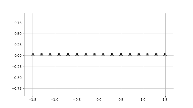
sfs.array.linear(N, spacing, center=[0, 0, 0], orientation=[1, 0, 0])

Linear secondary source distribution.

Parameters:

• N (int) – Number of secondary sources.
• spacing (float) – Distance (in metres) between secondary sources.
• center ((3,) array_like, optional) – Coordinates of array center.
• orientation ((3,) array_like, optional) – Orientation of the array. By default, the loudspeakers have their main axis pointing into positive x-direction.

Returns:

ArrayData – Positions, orientations and weights of secondary sources.

Examples

x0, n0, a0 = sfs.array.linear(16, 0.2, orientation=[0, -1, 0])
sfs.plot.loudspeaker_2d(x0, n0, a0)
plt.axis('equal')

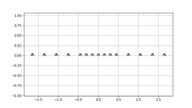
sfs.array.linear_diff(distances, center=[0, 0, 0], orientation=[1, 0, 0])

Linear secondary source distribution from a list of distances.

Parameters:

• distances ((N-1,) array_like) – Sequence of secondary sources distances in metres.
• center, orientation – See linear().

Returns:

ArrayData – Positions, orientations and weights of secondary sources.

Examples

x0, n0, a0 = sfs.array.linear_diff(4 * [0.3] + 6 * [0.15] + 4 * [0.3],
                                   orientation=[0, -1, 0])
sfs.plot.loudspeaker_2d(x0, n0, a0)
plt.axis('equal')

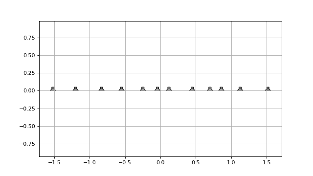
sfs.array.linear_random(N, min_spacing, max_spacing, center=[0, 0, 0], orientation=[1, 0, 0], seed=None)

Randomly sampled linear array.

Parameters:

• N (int) – Number of secondary sources.
• min_spacing, max_spacing (float) – Minimal and maximal distance (in metres) between secondary sources.
• center, orientation – See linear().
• seed ({None, int, array_like}, optional) – Random seed. See numpy.random.RandomState.

Returns:

ArrayData – Positions, orientations and weights of secondary sources.

Examples

x0, n0, a0 = sfs.array.linear_random(12, 0.15, 0.4, orientation=[0, -1, 0])
sfs.plot.loudspeaker_2d(x0, n0, a0)
plt.axis('equal')

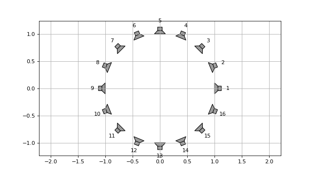
sfs.array.circular(N, R, center=[0, 0, 0])

Circular secondary source distribution parallel to the xy-plane.

Parameters:

• N (int) – Number of secondary sources.
• R (float) – Radius in metres.
• center – See linear().

Returns:

ArrayData – Positions, orientations and weights of secondary sources.

Examples

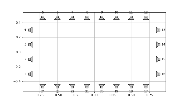
x0, n0, a0 = sfs.array.circular(16, 1)
sfs.plot.loudspeaker_2d(x0, n0, a0, size=0.2, show_numbers=True)
plt.axis('equal')

sfs.array.rectangular(N, spacing, center=[0, 0, 0], orientation=[1, 0, 0])

Rectangular secondary source distribution.

Parameters:

• N (int or pair of int) – Number of secondary sources on each side of the rectangle. If a pair of numbers is given, the first one specifies the first and third segment, the second number specifies the second and fourth segment.
• spacing (float) – Distance (in metres) between secondary sources.
• center, orientation – See linear(). The orientation corresponds to the first linear segment.

Returns:

ArrayData – Positions, orientations and weights of secondary sources.

Examples

x0, n0, a0 = sfs.array.rectangular((4, 8), 0.2)
sfs.plot.loudspeaker_2d(x0, n0, a0, show_numbers=True)
plt.axis('equal')

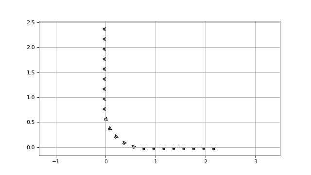
sfs.array.rounded_edge(Nxy, Nr, dx, center=[0, 0, 0], orientation=[1, 0, 0])

Array along the xy-axis with rounded edge at the origin.

Parameters:

• Nxy (int) – Number of secondary sources along x- and y-axis.
• Nr (int) – Number of secondary sources in rounded edge. Radius of edge is adjusted to equdistant sampling along entire array.
• center ((3,) array_like, optional) – Position of edge.
• orientation ((3,) array_like, optional) – Normal vector of array. Default orientation is along xy-axis.

Returns:

ArrayData – Positions, orientations and weights of secondary sources.

Examples

x0, n0, a0 = sfs.array.rounded_edge(8, 5, 0.2)
sfs.plot.loudspeaker_2d(x0, n0, a0)
plt.axis('equal')

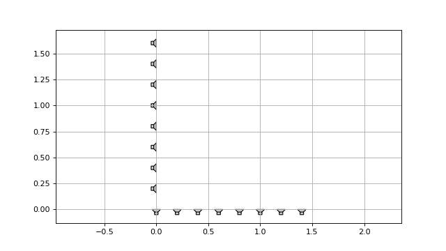
sfs.array.edge(Nxy, dx, center=[0, 0, 0], orientation=[1, 0, 0])

Array along the xy-axis with edge at the origin.

Parameters:

• Nxy (int) – Number of secondary sources along x- and y-axis.
• center ((3,) array_like, optional) – Position of edge.
• orientation ((3,) array_like, optional) – Normal vector of array. Default orientation is along xy-axis.

Returns:

ArrayData – Positions, orientations and weights of secondary sources.

Examples

x0, n0, a0 = sfs.array.edge(8, 0.2)
sfs.plot.loudspeaker_2d(x0, n0, a0)
plt.axis('equal')

sfs.array.planar(N, spacing, center=[0, 0, 0], orientation=[1, 0, 0])

Planar secondary source distribtion.

Parameters:

• N (int or pair of int) – Number of secondary sources along each edge. If a pair of numbers is given, the first one specifies the number on the horizontal edge, the second one specifies the number on the vertical edge.
• spacing (float) – Distance (in metres) between secondary sources.
• center, orientation – See linear().

Returns:

ArrayData – Positions, orientations and weights of secondary sources.

sfs.array.cube(N, spacing, center=[0, 0, 0], orientation=[1, 0, 0])

Cube-shaped secondary source distribtion.

Parameters:

• N (int or triple of int) – Number of secondary sources along each edge. If a triple of numbers is given, the first two specify the edges like in rectangular(), the last one specifies the vertical edge.
• spacing (float) – Distance (in metres) between secondary sources.
• center, orientation – See linear(). The orientation corresponds to the first planar segment.

Returns:

ArrayData – Positions, orientations and weights of secondary sources.

sfs.array.sphere_load(fname, radius, center=[0, 0, 0])

Spherical secondary source distribution loaded from datafile.

ASCII Format (see MATLAB SFS Toolbox) with 4 numbers (3 position, 1 weight) per secondary source located on the unit circle.

Returns:ArrayData – Positions, orientations and weights of secondary sources.

sfs.array.load(fname, center=[0, 0, 0], orientation=[1, 0, 0])

Load secondary source positions from datafile.

Comma Seperated Values (CSV) format with 7 values (3 positions, 3 normal vectors, 1 weight) per secondary source.

Returns:ArrayData – Positions, orientations and weights of secondary sources.

sfs.array.weights_midpoint(positions, closed)

Calculate loudspeaker weights for a simply connected array.

The weights are calculated according to the midpoint rule.

Parameters:

• positions ((N, 3) array_like) – Sequence of secondary source positions.

  Note

  The loudspeaker positions have to be ordered on the contour!

• closed (bool) – True if the loudspeaker contour is closed.

Returns:

(N,) numpy.ndarray – Weights of secondary sources.

sfs.array.concatenate(*arrays)

Concatenate ArrayData objects.

Tapering

Weights (tapering) for the driving function.

import sfs
import matplotlib.pyplot as plt
import numpy as np
plt.rcParams['figure.figsize'] = 8, 3  # inch
plt.rcParams['axes.grid'] = True

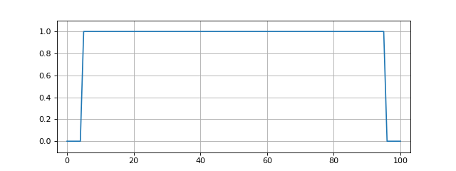
active1 = np.zeros(101, dtype=bool)
active1[5:-5] = True

# The active part can wrap around from the end to the beginning:
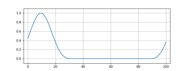
active2 = np.ones(101, dtype=bool)
active2[30:-10] = False

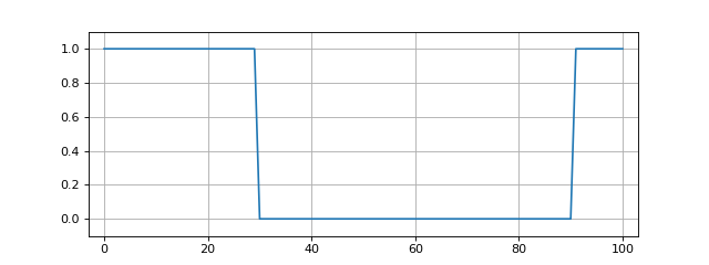
sfs.tapering.none(active)

No tapering window.

Parameters:active (array_like, dtype=bool) – A boolean array containing True for active loudspeakers. Returns:type(active) – The input, unchanged.

Examples

plt.plot(sfs.tapering.none(active1))
plt.axis([-3, 103, -0.1, 1.1])

plt.plot(sfs.tapering.none(active2))
plt.axis([-3, 103, -0.1, 1.1])

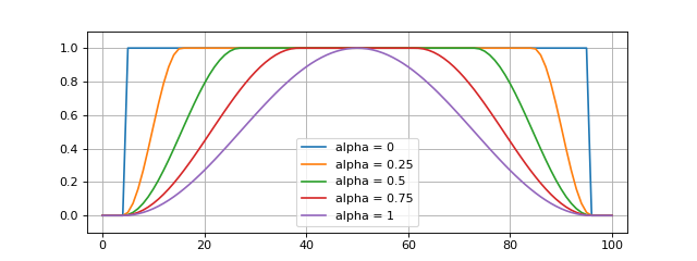
sfs.tapering.tukey(active, alpha)

Tukey tapering window.

This uses a function similar to scipy.signal.tukey(), except that the first and last value are not zero.

Parameters:

• active (array_like, dtype=bool) – A boolean array containing True for active loudspeakers.
• alpha (float) – Shape parameter of the Tukey window, see scipy.signal.tukey().

Returns:

(len(active),) numpy.ndarray – Tapering weights.

Examples

plt.plot(sfs.tapering.tukey(active1, 0), label='alpha = 0')
plt.plot(sfs.tapering.tukey(active1, 0.25), label='alpha = 0.25')
plt.plot(sfs.tapering.tukey(active1, 0.5), label='alpha = 0.5')
plt.plot(sfs.tapering.tukey(active1, 0.75), label='alpha = 0.75')
plt.plot(sfs.tapering.tukey(active1, 1), label='alpha = 1')
plt.axis([-3, 103, -0.1, 1.1])
plt.legend(loc='lower center')

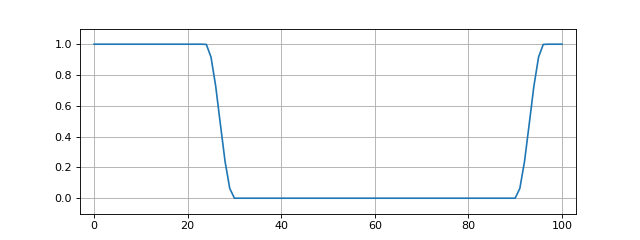
plt.plot(sfs.tapering.tukey(active2, 0.3))
plt.axis([-3, 103, -0.1, 1.1])

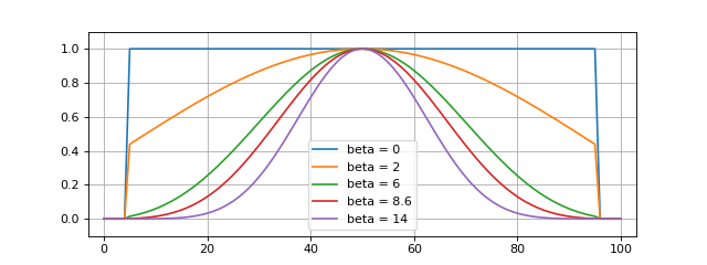
sfs.tapering.kaiser(active, beta)

Kaiser tapering window.

This uses numpy.kaiser().

Parameters:

• active (array_like, dtype=bool) – A boolean array containing True for active loudspeakers.
• alpha (float) – Shape parameter of the Kaiser window, see numpy.kaiser().

Returns:

(len(active),) numpy.ndarray – Tapering weights.

Examples

plt.plot(sfs.tapering.kaiser(active1, 0), label='beta = 0')
plt.plot(sfs.tapering.kaiser(active1, 2), label='beta = 2')
plt.plot(sfs.tapering.kaiser(active1, 6), label='beta = 6')
plt.plot(sfs.tapering.kaiser(active1, 8.6), label='beta = 8.6')
plt.plot(sfs.tapering.kaiser(active1, 14), label='beta = 14')
plt.axis([-3, 103, -0.1, 1.1])
plt.legend(loc='lower center')

plt.plot(sfs.tapering.kaiser(active2, 7))
plt.axis([-3, 103, -0.1, 1.1])