Modal Room Acoustics
In [1]:
import numpy as np
import matplotlib.pyplot as plt
import sfs
/home/docs/checkouts/readthedocs.org/user_builds/sfs-python/conda/0.4.0/lib/python3.5/importlib/_bootstrap.py:222: RuntimeWarning: numpy.dtype size changed, may indicate binary incompatibility. Expected 96, got 88
  return f(*args, **kwds)
In [2]:
%matplotlib inline
In [3]:
x0 = 1, 3, 1.80  # source position
L = 6, 6, 3  # dimensions of room
deltan = 0.01  # absorption factor of walls
n0 = 1, 0, 0  # normal vector of source (only for compatibility)
N = 20  # maximum order of modes
You can experiment with different combinations of modes:
In [4]:
#N = [[1], 0, 0]
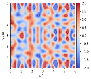
Sound Field for One Frequency
In [5]:
f = 500  # frequency
omega = 2 * np.pi * f  # angular frequency
In [6]:
grid = sfs.util.xyz_grid([0, L[0]], [0, L[1]], L[2] / 2, spacing=.1)
In [7]:
p = sfs.mono.source.point_modal(omega, x0, n0, grid, L, N=N, deltan=deltan)
For now, we apply an arbitrary scaling factor to make the plot look good
TODO: proper normalization
In [8]:
p *= 0.05
In [9]:
sfs.plot.soundfield(p, grid);
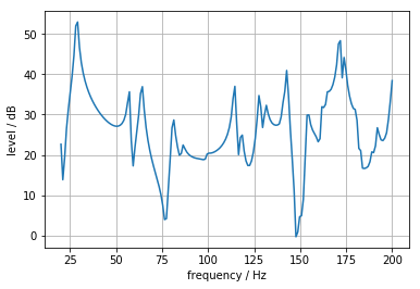
Frequency Response at One Point
In [10]:
f = np.linspace(20, 200, 180)  # frequency
omega = 2 * np.pi * f  # angular frequency

receiver = 1, 1, 1.8

p = [sfs.mono.source.point_modal(om, x0, n0, receiver, L, N=N, deltan=deltan)
     for om in omega]

plt.plot(f, sfs.util.db(p))
plt.xlabel('frequency / Hz')
plt.ylabel('level / dB')
plt.grid()