Frequency Domain
Submodules for monochromatic sound fields.
Monochromatic Sources
Compute the sound field generated by a sound source.
import sfs
import numpy as np
import matplotlib.pyplot as plt
plt.rcParams['figure.figsize'] = 8, 4.5  # inch

x0 = 1.5, 1, 0
f = 500  # Hz
omega = 2 * np.pi * f

normalization_point = 4 * np.pi
normalization_line = \
    np.sqrt(8 * np.pi * omega / sfs.defs.c) * np.exp(1j * np.pi / 4)

grid = sfs.util.xyz_grid([-2, 3], [-1, 2], 0, spacing=0.02)

# Grid for vector fields:
vgrid = sfs.util.xyz_grid([-2, 3], [-1, 2], 0, spacing=0.1)
-
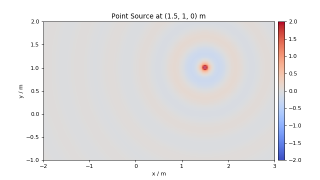
sfs.mono.source.point(omega, x0, n0, grid, c=None)[source]¶ Point source.
Notes
              1  e^(-j w/c |x-x0|)
G(x-x0, w) = --- -----------------
             4pi      |x-x0|
Examples
p = sfs.mono.source.point(omega, x0, None, grid)
sfs.plot.soundfield(p, grid)
plt.title("Point Source at {} m".format(x0))
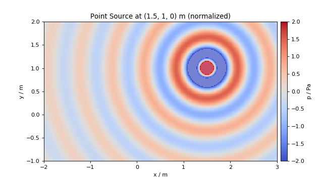
Normalization …
sfs.plot.soundfield(p * normalization_point, grid,
                    colorbar_kwargs=dict(label="p / Pa"))
plt.title("Point Source at {} m (normalized)".format(x0))
-
sfs.mono.source.point_velocity(omega, x0, n0, grid, c=None)[source]¶ Velocity of a point source.
Returns: XyzComponents– Particle velocity at positions given by grid.Examples
The particle velocity can be plotted on top of the sound pressure:
v = sfs.mono.source.point_velocity(omega, x0, None, vgrid)
sfs.plot.soundfield(p * normalization_point, grid)
sfs.plot.vectors(v * normalization_point, vgrid)
plt.title("Sound Pressure and Particle Velocity")

-
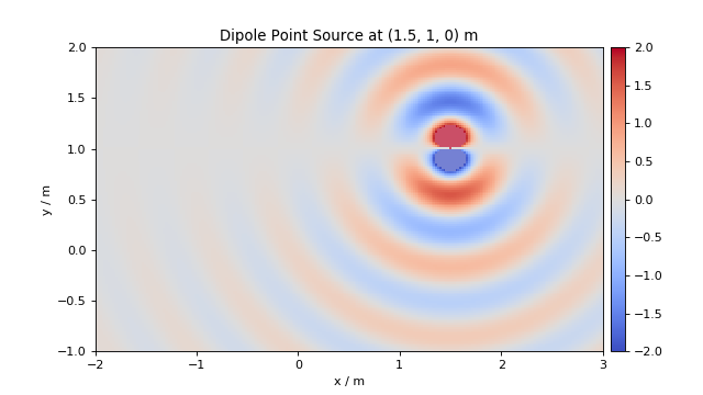
sfs.mono.source.point_dipole(omega, x0, n0, grid, c=None)[source]¶ Point source with dipole characteristics.
Parameters: - omega (float) – Frequency of source.
- x0 ((3,) array_like) – Position of source.
- n0 ((3,) array_like) – Normal vector (direction) of dipole.
- grid (triple of array_like) – The grid that is used for the sound field calculations.
See
sfs.util.xyz_grid(). - c (float, optional) – Speed of sound.
Returns: numpy.ndarray – Sound pressure at positions given by grid.
Notes
 d                1   / iw       1    \   (x-x0) n0
---- G(x-x0,w) = --- | ----- + ------- | ----------- e^(-i w/c |x-x0|)
d ns             4pi  \  c     |x-x0| /   |x-x0|^2
Examples
n0 = 0, 1, 0
p = sfs.mono.source.point_dipole(omega, x0, n0, grid)
sfs.plot.soundfield(p, grid)
plt.title("Dipole Point Source at {} m".format(x0))
-
sfs.mono.source.point_modal(omega, x0, n0, grid, L, N=None, deltan=0, c=None)[source]¶ Point source in a rectangular room using a modal room model.
Parameters: - omega (float) – Frequency of source.
- x0 ((3,) array_like) – Position of source.
- n0 ((3,) array_like) – Normal vector (direction) of source (only required for compatibility).
- grid (triple of array_like) – The grid that is used for the sound field calculations.
See
sfs.util.xyz_grid(). - L ((3,) array_like) – Dimensionons of the rectangular room.
- N ((3,) array_like or int, optional) – For all three spatial dimensions per dimension maximum order or list of orders. A scalar applies to all three dimensions. If no order is provided it is approximately determined.
- deltan (float, optional) – Absorption coefficient of the walls.
- c (float, optional) – Speed of sound.
Returns: numpy.ndarray – Sound pressure at positions given by grid.
-
sfs.mono.source.point_modal_velocity(omega, x0, n0, grid, L, N=None, deltan=0, c=None)[source]¶ Velocity of point source in a rectangular room using a modal room model.
Parameters: - omega (float) – Frequency of source.
- x0 ((3,) array_like) – Position of source.
- n0 ((3,) array_like) – Normal vector (direction) of source (only required for compatibility).
- grid (triple of array_like) – The grid that is used for the sound field calculations.
See
sfs.util.xyz_grid(). - L ((3,) array_like) – Dimensionons of the rectangular room.
- N ((3,) array_like or int, optional) – Combination of modal orders in the three-spatial dimensions to calculate the sound field for or maximum order for all dimensions. If not given, the maximum modal order is approximately determined and the sound field is computed up to this maximum order.
- deltan (float, optional) – Absorption coefficient of the walls.
- c (float, optional) – Speed of sound.
Returns: XyzComponents– Particle velocity at positions given by grid.
-
sfs.mono.source.point_image_sources(omega, x0, n0, grid, L, max_order, coeffs=None, c=None)[source]¶ Point source in a rectangular room using the mirror image source model.
Parameters: - omega (float) – Frequency of source.
- x0 ((3,) array_like) – Position of source.
- n0 ((3,) array_like) – Normal vector (direction) of source (only required for compatibility).
- grid (triple of array_like) – The grid that is used for the sound field calculations.
See
sfs.util.xyz_grid(). - L ((3,) array_like) – Dimensions of the rectangular room.
- max_order (int) – Maximum number of reflections for each image source.
- coeffs ((6,) array_like, optional) – Reflection coeffecients of the walls. If not given, the reflection coefficients are set to one.
- c (float, optional) – Speed of sound.
Returns: numpy.ndarray – Sound pressure at positions given by grid.
-
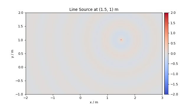
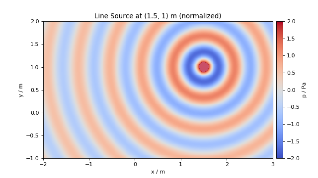
sfs.mono.source.line(omega, x0, n0, grid, c=None)[source]¶ Line source parallel to the z-axis.
Note: third component of x0 is ignored.
Notes
                   (2)
G(x-x0, w) = -j/4 H0  (w/c |x-x0|)
Examples
p = sfs.mono.source.line(omega, x0, None, grid)
sfs.plot.soundfield(p, grid)
plt.title("Line Source at {} m".format(x0[:2]))
Normalization …
sfs.plot.soundfield(p * normalization_line, grid,
                    colorbar_kwargs=dict(label="p / Pa"))
plt.title("Line Source at {} m (normalized)".format(x0[:2]))
-
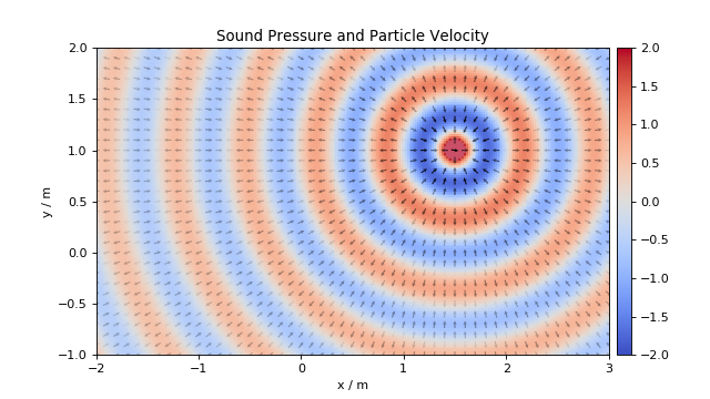
sfs.mono.source.line_velocity(omega, x0, n0, grid, c=None)[source]¶ Velocity of line source parallel to the z-axis.
Returns: XyzComponents– Particle velocity at positions given by grid.Examples
The particle velocity can be plotted on top of the sound pressure:
v = sfs.mono.source.line_velocity(omega, x0, None, vgrid)
sfs.plot.soundfield(p * normalization_line, grid)
sfs.plot.vectors(v * normalization_line, vgrid)
plt.title("Sound Pressure and Particle Velocity")
-
sfs.mono.source.line_dipole(omega, x0, n0, grid, c=None)[source]¶ Line source with dipole characteristics parallel to the z-axis.
Note: third component of x0 is ignored.
Notes
                   (2)
G(x-x0, w) = jk/4 H1  (w/c |x-x0|) cos(phi)
-
sfs.mono.source.line_dirichlet_edge(omega, x0, grid, alpha=4.71238898038469, Nc=None, c=None)[source]¶ Line source scattered at an edge with Dirichlet boundary conditions.
[Mos12], eq.(10.18/19)
Parameters: - omega (float) – Angular frequency.
- x0 ((3,) array_like) – Position of line source.
- grid (triple of array_like) – The grid that is used for the sound field calculations.
See
sfs.util.xyz_grid(). - alpha (float, optional) – Outer angle of edge.
- Nc (int, optional) – Number of elements for series expansion of driving function. Estimated if not given.
- c (float, optional) – Speed of sound
Returns: numpy.ndarray – Complex pressure at grid positions.
-
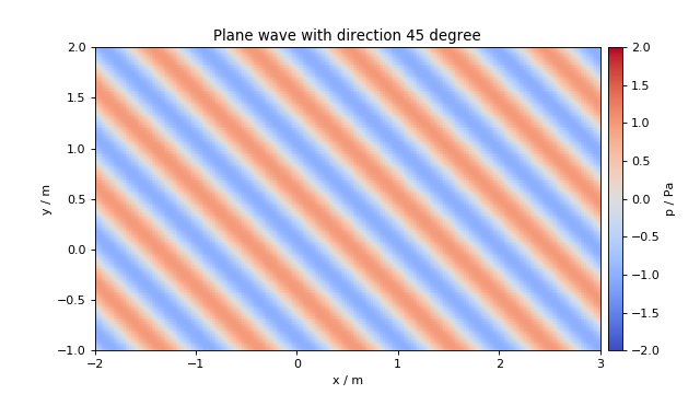
sfs.mono.source.plane(omega, x0, n0, grid, c=None)[source]¶ Plane wave.
Notes
G(x, w) = e^(-i w/c n x)
Examples
direction = 45  # degree
n0 = sfs.util.direction_vector(np.radians(direction))
p = sfs.mono.source.plane(omega, x0, n0, grid)
sfs.plot.soundfield(p, grid, colorbar_kwargs=dict(label="p / Pa"))
plt.title("Plane wave with direction {} degree".format(direction))
-
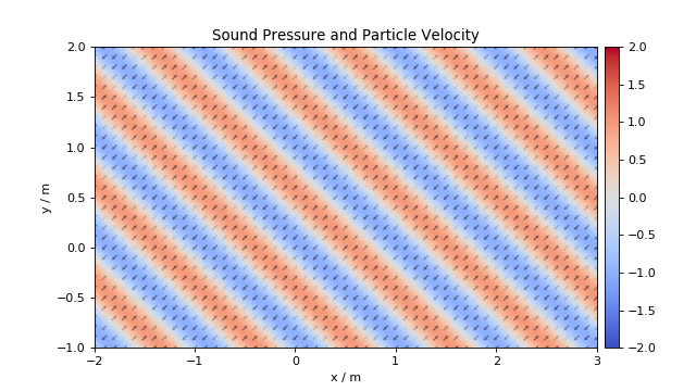
sfs.mono.source.plane_velocity(omega, x0, n0, grid, c=None)[source]¶ Velocity of a plane wave.
Notes
V(x, w) = 1/(rho c) e^(-i w/c n x) n
Returns: XyzComponents– Particle velocity at positions given by grid.Examples
The particle velocity can be plotted on top of the sound pressure:
v = sfs.mono.source.plane_velocity(omega, x0, n0, vgrid)
sfs.plot.soundfield(p, grid)
sfs.plot.vectors(v, vgrid)
plt.title("Sound Pressure and Particle Velocity")
Monochromatic Driving Functions
Compute driving functions for various systems.
-
sfs.mono.drivingfunction.wfs_2d_line(omega, x0, n0, xs, c=None)[source]¶ Line source by 2-dimensional WFS.
D(x0,k) = j/2 k (x0-xs) n0 / |x0-xs| * H1(k |x0-xs|)
-
sfs.mono.drivingfunction.wfs_2d_point(omega, x0, n0, xs, c=None)¶ Point source by two- or three-dimensional WFS.
               (x0-xs) n0
D(x0,k) = j k ------------- e^(-j k |x0-xs|)
              |x0-xs|^(3/2)
-
sfs.mono.drivingfunction.wfs_25d_point(omega, x0, n0, xs, xref=[0, 0, 0], c=None, omalias=None)[source]¶ Point source by 2.5-dimensional WFS.
            ____________   (x0-xs) n0
D(x0,k) = \|j k |xref-x0| ------------- e^(-j k |x0-xs|)
                          |x0-xs|^(3/2)
-
sfs.mono.drivingfunction.wfs_3d_point(omega, x0, n0, xs, c=None)¶ Point source by two- or three-dimensional WFS.
               (x0-xs) n0
D(x0,k) = j k ------------- e^(-j k |x0-xs|)
              |x0-xs|^(3/2)
-
sfs.mono.drivingfunction.wfs_2d_plane(omega, x0, n0, n=[0, 1, 0], c=None)¶ Plane wave by two- or three-dimensional WFS.
Eq.(17) from [SRA08]:
D(x0,k) = j k n n0 e^(-j k n x0)
-
sfs.mono.drivingfunction.wfs_25d_plane(omega, x0, n0, n=[0, 1, 0], xref=[0, 0, 0], c=None, omalias=None)[source]¶ Plane wave by 2.5-dimensional WFS.
                 ____________
D_2.5D(x0,w) = \|j k |xref-x0| n n0 e^(-j k n x0)
-
sfs.mono.drivingfunction.wfs_3d_plane(omega, x0, n0, n=[0, 1, 0], c=None)¶ Plane wave by two- or three-dimensional WFS.
Eq.(17) from [SRA08]:
D(x0,k) = j k n n0 e^(-j k n x0)
-
sfs.mono.drivingfunction.wfs_2d_focused(omega, x0, n0, xs, c=None)¶ Focused source by two- or three-dimensional WFS.
               (x0-xs) n0
D(x0,k) = j k ------------- e^(j k |x0-xs|)
              |x0-xs|^(3/2)
-
sfs.mono.drivingfunction.wfs_25d_focused(omega, x0, n0, xs, xref=[0, 0, 0], c=None, omalias=None)[source]¶ Focused source by 2.5-dimensional WFS.
            ____________   (x0-xs) n0
D(x0,w) = \|j k |xref-x0| ------------- e^(j k |x0-xs|)
                          |x0-xs|^(3/2)
-
sfs.mono.drivingfunction.wfs_3d_focused(omega, x0, n0, xs, c=None)¶ Focused source by two- or three-dimensional WFS.
               (x0-xs) n0
D(x0,k) = j k ------------- e^(j k |x0-xs|)
              |x0-xs|^(3/2)
-
sfs.mono.drivingfunction.delay_3d_plane(omega, x0, n0, n=[0, 1, 0], c=None)[source]¶ Plane wave by simple delay of secondary sources.
-
sfs.mono.drivingfunction.source_selection_plane(n0, n)[source]¶ Secondary source selection for a plane wave.
Eq.(13) from [SRA08]
-
sfs.mono.drivingfunction.source_selection_point(n0, x0, xs)[source]¶ Secondary source selection for a point source.
Eq.(15) from [SRA08]
-
sfs.mono.drivingfunction.source_selection_line(n0, x0, xs)[source]¶ Secondary source selection for a line source.
compare Eq.(15) from [SRA08]
-
sfs.mono.drivingfunction.source_selection_focused(ns, x0, xs)[source]¶ Secondary source selection for a focused source.
Eq.(2.78) from [Wie14]
-
sfs.mono.drivingfunction.nfchoa_2d_plane(omega, x0, r0, n=[0, 1, 0], max_order=None, c=None)[source]¶ Plane wave by two-dimensional NFC-HOA.
\[D(\phi_0, \omega) = -\frac{2\i}{\pi r_0} \sum_{m=-M}^M \frac{\i^{-m}}{\Hankel{2}{m}{\wc r_0}} \e{\i m (\phi_0 - \phi_\text{pw})}\]
-
sfs.mono.drivingfunction.nfchoa_25d_point(omega, x0, r0, xs, max_order=None, c=None)[source]¶ Point source by 2.5-dimensional NFC-HOA.
\[D(\phi_0, \omega) = \frac{1}{2 \pi r_0} \sum_{m=-M}^M \frac{\hankel{2}{|m|}{\wc r}}{\hankel{2}{|m|}{\wc r_0}} \e{\i m (\phi_0 - \phi)}\]
-
sfs.mono.drivingfunction.nfchoa_25d_plane(omega, x0, r0, n=[0, 1, 0], max_order=None, c=None)[source]¶ Plane wave by 2.5-dimensional NFC-HOA.
\[D(\phi_0, \omega) = \frac{2\i}{r_0} \sum_{m=-M}^M \frac{\i^{-|m|}}{\wc \hankel{2}{|m|}{\wc r_0}} \e{\i m (\phi_0 - \phi_\text{pw})}\]
-
sfs.mono.drivingfunction.sdm_2d_line(omega, x0, n0, xs, c=None)[source]¶ Line source by two-dimensional SDM.
The secondary sources have to be located on the x-axis (y0=0). Derived from [SA09], Eq.(9), Eq.(4):
D(x0,k) =
-
sfs.mono.drivingfunction.sdm_2d_plane(omega, x0, n0, n=[0, 1, 0], c=None)[source]¶ Plane wave by two-dimensional SDM.
The secondary sources have to be located on the x-axis (y0=0). Derived from [Ahr12], Eq.(3.73), Eq.(C.5), Eq.(C.11):
D(x0,k) = kpw,y * e^(-j*kpw,x*x)
-
sfs.mono.drivingfunction.sdm_25d_plane(omega, x0, n0, n=[0, 1, 0], xref=[0, 0, 0], c=None)[source]¶ Plane wave by 2.5-dimensional SDM.
The secondary sources have to be located on the x-axis (y0=0). Eq.(3.79) from [Ahr12]:
D_2.5D(x0,w) =
-
sfs.mono.drivingfunction.sdm_25d_point(omega, x0, n0, xs, xref=[0, 0, 0], c=None)[source]¶ Point source by 2.5-dimensional SDM.
The secondary sources have to be located on the x-axis (y0=0). Driving funcnction from [SA10], Eq.(24):
D(x0,k) =
-
sfs.mono.drivingfunction.esa_edge_2d_plane(omega, x0, n=[0, 1, 0], alpha=4.71238898038469, Nc=None, c=None)[source]¶ - Plane wave by two-dimensional ESA for an edge-shaped secondary source
- distribution consisting of monopole line sources.
One leg of the secondary sources has to be located on the x-axis (y0=0), the edge at the origin.
Derived from [SSR16]
Parameters: - omega (float) – Angular frequency.
- x0 (int(N, 3) array_like) – Sequence of secondary source positions.
- n ((3,) array_like, optional) – Normal vector of synthesized plane wave.
- alpha (float, optional) – Outer angle of edge.
- Nc (int, optional) – Number of elements for series expansion of driving function. Estimated if not given.
- c (float, optional) – Speed of sound
Returns: (N,) numpy.ndarray – Complex weights of secondary sources.
-
sfs.mono.drivingfunction.esa_edge_dipole_2d_plane(omega, x0, n=[0, 1, 0], alpha=4.71238898038469, Nc=None, c=None)[source]¶ - Plane wave by two-dimensional ESA for an edge-shaped secondary source
- distribution consisting of dipole line sources.
One leg of the secondary sources has to be located on the x-axis (y0=0), the edge at the origin.
Derived from [SSR16]
Parameters: - omega (float) – Angular frequency.
- x0 (int(N, 3) array_like) – Sequence of secondary source positions.
- n ((3,) array_like, optional) – Normal vector of synthesized plane wave.
- alpha (float, optional) – Outer angle of edge.
- Nc (int, optional) – Number of elements for series expansion of driving function. Estimated if not given.
- c (float, optional) – Speed of sound
Returns: (N,) numpy.ndarray – Complex weights of secondary sources.
-
sfs.mono.drivingfunction.esa_edge_2d_line(omega, x0, xs, alpha=4.71238898038469, Nc=None, c=None)[source]¶ - Line source by two-dimensional ESA for an edge-shaped secondary source
- distribution constisting of monopole line sources.
One leg of the secondary sources have to be located on the x-axis (y0=0), the edge at the origin.
Derived from [SSR16]
Parameters: - omega (float) – Angular frequency.
- x0 (int(N, 3) array_like) – Sequence of secondary source positions.
- xs ((3,) array_like) – Position of synthesized line source.
- alpha (float, optional) – Outer angle of edge.
- Nc (int, optional) – Number of elements for series expansion of driving function. Estimated if not given.
- c (float, optional) – Speed of sound
Returns: (N,) numpy.ndarray – Complex weights of secondary sources.
-
sfs.mono.drivingfunction.esa_edge_25d_point(omega, x0, xs, xref=[2, -2, 0], alpha=4.71238898038469, Nc=None, c=None)[source]¶ - Point source by 2.5-dimensional ESA for an edge-shaped secondary source
- distribution constisting of monopole line sources.
One leg of the secondary sources have to be located on the x-axis (y0=0), the edge at the origin.
Derived from [SSR16]
Parameters: - omega (float) – Angular frequency.
- x0 (int(N, 3) array_like) – Sequence of secondary source positions.
- xs ((3,) array_like) – Position of synthesized line source.
- xref ((3,) array_like or float) – Reference position or reference distance
- alpha (float, optional) – Outer angle of edge.
- Nc (int, optional) – Number of elements for series expansion of driving function. Estimated if not given.
- c (float, optional) – Speed of sound
Returns: (N,) numpy.ndarray – Complex weights of secondary sources.
-
sfs.mono.drivingfunction.esa_edge_dipole_2d_line(omega, x0, xs, alpha=4.71238898038469, Nc=None, c=None)[source]¶ - Line source by two-dimensional ESA for an edge-shaped secondary source
- distribution constisting of dipole line sources.
One leg of the secondary sources have to be located on the x-axis (y0=0), the edge at the origin.
Derived from [SSR16]
Parameters: - omega (float) – Angular frequency.
- x0 ((N, 3) array_like) – Sequence of secondary source positions.
- xs ((3,) array_like) – Position of synthesized line source.
- alpha (float, optional) – Outer angle of edge.
- Nc (int, optional) – Number of elements for series expansion of driving function. Estimated if not given.
- c (float, optional) – Speed of sound
Returns: (N,) numpy.ndarray – Complex weights of secondary sources.